
Stellar astrophysics Created 2026-09-24 Updated 2026-09-24
Stellar astrophysics studies the structure, formation, energy production, observable properties, and evolution of stars.
Planetary science Created 2026-09-24 Updated 2026-11-05
Planetary science explains the formation, structure and evolution of planets, their natural satellites and smaller bodies by connecting observations with physical and chemical models. A body's mass and radius constrain its mean density, but several mixtures and interior structures can fit the same pair of measurements.
Spectroscopy probes accessible surface or atmospheric composition, gravity measurements constrain internal mass distribution, and seismic waves probe elastic layers. Comparing these independent observations tests models of differentiation, cooling, planet formation and atmospheric evolution. Nearby Solar-system bodies also provide resolved examples for interpreting the limited signals available from an exoplanet.
Radiative transfer Created 2026-09-24 Updated 2026-11-05
Radiative transfer follows how emission, absorption and scattering change specific intensity. Along a ray, the radiative transfer equation has the formwhere adds radiation and removes it from the ray. Scattering into the ray can couple this equation to other directions.
The optical depth measures attenuation along a path; the source function compares emission with extinction. Their variation explains why spectral lines probe different depths of a stellar atmosphere rather than a single emitting surface.[ref]
Radiative Transfer in Stellar Atmospheres by Robert J. Rutten (8th edition). §2.2, equations (2.25)–(2.26): transfer along a ray and the source-function description
Exoplanet Created 2026-09-24 Updated 2026-10-18
An exoplanet is a planet outside the Solar system; here the focus is on planets orbiting stars other than the Sun, including pulsars. Most exoplanets are detected indirectly: a star's changing Doppler shift reveals its motion, or a small dip in its light curve reveals an exoplanet transit. The striking idea is that an unresolved point of light can tell us about an otherwise unseen world's mass, radius, and orbit.
The measurements answer different questions. Exoplanet transit photometry primarily gives a radius ratio, while Doppler spectroscopy constrains mass together with orbital inclination. Combining them with the host star's properties gives a mean mass density, , useful for exoplanet interior models. Even this combination does not uniquely determine composition: see exoplanet interior-composition degeneracy. Transit spectroscopy and an exoplanet secondary eclipse then probe an exoplanet atmosphere.
The discovery history has two distinct milestones. In 1992 Aleksander Wolszczan and Dale Frail reported two planet-mass companions to the pulsar PSR B1257+12 from periodic changes in pulse arrival times; their paper also suggested an additional companion. These were the first confirmed exoplanet discoveries, around a neutron star. [ref]
https://www.nature.com/articles/355145a0. Wolszczan and Frail (1992)
. Wolszczan's contemporary conference account, archived by NASA, likewise distinguishes the two reported companions from a possible third. [ref]https://ntrs.nasa.gov/citations/19920021993. Wolszczan (1992), NASA archive
.In 1995 Michel Mayor and Didier Queloz discovered 51 Pegasi b through Doppler spectroscopy, the landmark first confirmed exoplanet around a Sun-like star. This was a hot Jupiter, not the first exoplanet of every kind: the earlier pulsar discoveries belong to a different host category. [ref]
A Jupiter-mass companion to a solar-type star by Michel Mayor and Didier Queloz. Mayor and Queloz (1995)
. NASA's contemporary account describes the confirmation and the approximately four-day orbital period. [ref]https://science.nasa.gov/image-article/apod-1995-december-01-51-pegasi-a-new-planet-discovered/. NASA account (December 1995)
. Non-Archimedean analysis Created 2026-09-24 Updated 2026-11-05
Non-Archimedean analysis studies fields equipped with an Non-Archimedean absolute value, satisfying . The main examples are the P-adic numbers and fields of Laurent series field.
For example, in the 2-adic metric, and are extremely close because their difference is divisible by a high power of two. The inequality makes every triangle isosceles with the two larger sides equal. Over a complete non-Archimedean field, a series converges exactly when its terms tend to zero, a stronger conclusion than in ordinary real analysis. The subject makes congruence information accessible to methods involving limits, derivatives, and power series.
Arithmetic progression Created 2026-09-24 Updated 2026-10-18
An arithmetic progression is a sequence with a constant common difference between consecutive sequence terms. It has the form and is nonconstant when . Using for the common difference and numbering the first sequence term as , its explicit and recursive descriptions areThe explicit formula reaches any position directly; the recurrence reaches the next position from the current one. The factor counts the steps after the first entry. For real , a positive common difference makes the sequence increase, a negative one makes it decrease, and zero makes it constant.[ref]
11.2 Arithmetic Sequences. Precalculus 2e, §11.2 Arithmetic Sequences: definition, Recursive Formula for an Arithmetic Sequence and Explicit Formula for an Arithmetic Sequence
For an original example, start at seven and add three each time:The eighth entry is : eight sequence terms require seven increments. This counting principle makes arithmetic progressions useful for regularly spaced positions, repeated equal additions, and iteration over evenly spaced integers. The values need not be integers; starting at with common difference gives .
A geometric progression instead holds a ratio constant. In the displayed arithmetic progression, and differ even though . Multiplying each entry by two would give a different kind of repeated update from adding three. Distinguishing the two rules matters before predicting later entries or adding the sequence terms.
Equal differences also appear in Nicomachus's treatment of arithmetic proportion. He describes successions of at least three numbers whose neighboring differences agree, then explains how regularly omitting counting numbers changes the common gap. This connects the progression to the arithmetic mean: a middle entry is equally far from its two neighbors.[ref]
Multiplication Created 2026-09-24 Updated 2026-10-13
Multiplication combines two factors into their product of numbers. For a natural number , is the sum of copies of ; with no copies the result is zero. This repeated-addition interpretation directly explains integer grouping, while multiplication of arbitrary real numbers also describes scaling by noninteger factors.
A rectangle of side lengths and has area . Split the second side into lengths and . The two areas are and , giving the visible identityRotating the same rectangle interchanges the sides without changing its area, explaining . These pictures illustrate distributivity and commutativity for ordinary positive numbers; matrix multiplication and other operations require their own rules.
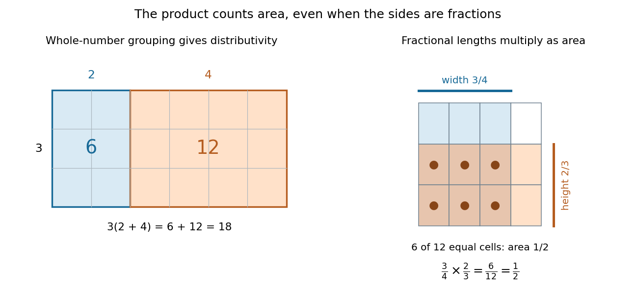
Partitioning a rectangle explains distributivity; partitioning a unit square gives an exact product of fractions
. Details. 
For a fractional example, take of a quantity and then of that result: the combined scale is . The two fractions are multiplicative inverses. In the unit square on the right, the overlap of a strip occupying of the width with one occupying of the height contains six of twelve equal cells. Its area is . The product stays exact even though the decimal expansion of repeats. [ref]
https://openstax.org/books/prealgebra-2e/pages/4-1-visualize-fractions. OpenStax, Prealgebra 2e, equal-part models of fractions
Subtraction Created 2026-09-24 Updated 2026-10-13
Subtraction adds the additive inverse: . On the number line, is a shift three units left from . Reversing the two inputs changes the sign: , so subtraction is generally not commutative. Solving gives the same answer by adding to both sides; the operation preserves equality while undoing the added amount.
Addition Created 2026-09-24 Updated 2026-10-13
Addition combines two numbers into their sum. For natural numbers, joining disjoint collections of sizes gives a collection of size . On a number line, adding shifts a starting position by : rightward when and leftward when .
Starting at and adding reaches . Starting there and adding returns to , because . Additive inverses turn this return move into an algebraic rule. With real numbers, addition is commutative and associative: exchanging two shifts or grouping several shifts differently leaves the final position unchanged.
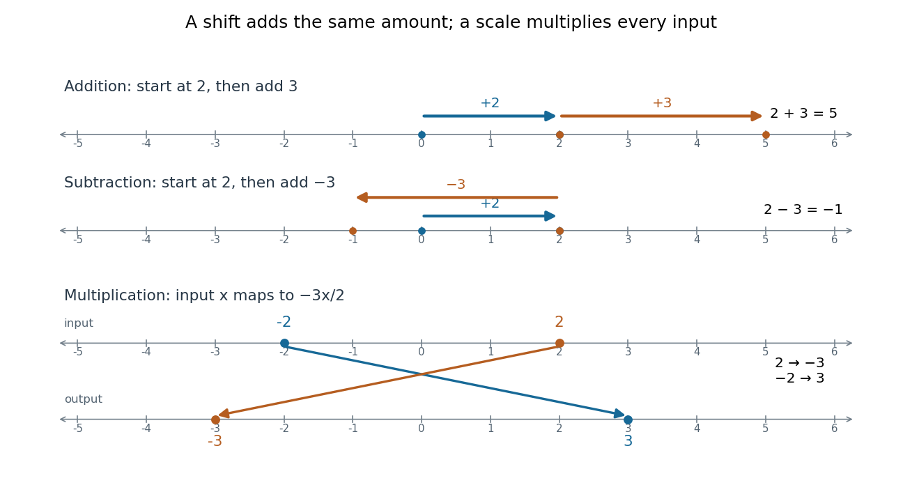
Addition shifts positions on a number line, while a negative multiplication factor changes both scale and direction
. Details. 
The bottom panel applies . Input becomes , and input becomes . Multiplication by a negative real number rescales distances from zero and reverses direction, giving a reflection in mathematics as well as a scale change. This is a different operation from shifting every input by one fixed amount.
Real number Created 2026-09-24 Updated 2026-11-05
A real number is an element of the complete ordered field . This includes integers, rational numbers such as , and irrational numbers such as . The number line represents each real number by a point, and the total order distinguishes which of two different points is larger.
The field operations permit addition, subtraction, multiplication and division by nonzero real numbers. Completeness adds the least-upper-bound property: every nonempty set of real numbers that is bounded above has a supremum in . For example, the positive real numbers whose squares are less than two have supremum . That supremum is not a rational number, illustrating why the rational numbers alone leave a gap.
The density of the rational numbers means every real number can be approximated arbitrarily closely by rational numbers. Constructions through Cauchy sequences or Dedekind cuts make those approximations into a precise description of .
Natural number Created 2026-09-24 Updated 2026-11-05
The natural numbers are the nonnegative integersThey count the elements of finite sets: the empty set has cardinality zero, and a two-element set has cardinality two. Addition and multiplication preserve natural numbers, while subtraction need not: is an integer outside .
The convention here includes zero. The positive integers instead begin at one. The well-ordering principle for the natural numbers ensures every nonempty subset has a least element, supporting mathematical induction and proof by minimal counterexample.
Uniform approximation Created 2026-09-24 Updated 2026-10-14
Uniform approximation minimizes the supremum norm of the difference between a target function and an approximant.
The error is measured uniformly over the domain using the supremum norm. A sequence of approximants whose uniform error tends to zero converges by uniform convergence; the optimization problem and the convergence notion are distinct.
Fixed-point theorem Created 2026-09-24 Updated 2026-10-14
Calculus of variations Created 2026-09-24 Updated 2026-11-05
The calculus of variations studies functionals whose inputs are functions, curves or fields. A variational problem specifies an admissible class, including endpoint or other boundary conditions, and asks for stationary points or minimizers. The first variation gives an equation for stationary candidates; a second variation, convexity or a direct comparison is needed to decide minimality.
For example, minimizeA zero-endpoint variation gives . If is twice differentiable, integration by parts and the fundamental lemma of the calculus of variations yield . The candidate is the straight line .
It is also the unique global minimizer, not merely stationary. Write any admissible with zero endpoint values for . The cross term is , soEquality forces . This argument extends to Sobolev spaces with a meaningful endpoint trace and illustrates the Dirichlet principle. In more complicated problems, the direct method in the calculus of variations establishes existence without first solving the stationarity equation.
Distribution theory Created 2026-09-24 Updated 2026-11-05
Distribution theory extends ordinary functions by letting them act on smooth test functions. A locally integrable function acts by , while the Dirac delta distribution acts by . The latter is a point source, rather than an ordinary function with a very large value. The space of test functions and its topology make distributions continuous linear functionals.[ref]
Partial Differential Equations by John K. Hunter. Chapter3, sections3.1–3.3, weak derivatives and distributions
Integration by parts supplies a distributional derivative even when ordinary differentiability fails:For the Heaviside function , , so . A jump has become a point source under differentiation. This is useful for impulses in differential equations, concentrated loads and interface jump conditions.
The extension has limits: multiplying a distribution by a smooth function is always defined, but arbitrary products of distributions are not. The theory controls which operations are meaningful through their action on test functions, rather than by manipulating symbolic point values.
Partial differential equation Created 2026-09-24 Updated 2026-10-14
A partial differential equation relates an unknown function of several independent variables to its partial derivatives. For , the notation means changing time while holding position fixed; measures how its spatial slope changes. Unlike an ordinary differential equation, a partial differential equation can describe an entire evolving profile rather than a single trajectory.
The heat equation smooths spatial variations, the transport equation moves them, and Laplace's equation describes a spatial equilibrium. Here is a diffusivity, is a velocity, and is the Laplacian. The periodic heat and transport comparison makes the difference visible using identical initial conditions.
A partial differential equation usually supplies a local rule rather than a complete answer. For example, every satisfies the heat equation with zero PDE source term; data select which profile is relevant. A complete problem specifies its domain of a function, coefficients, initial conditions, boundary conditions, and meaning of solution of a partial differential equation. A well-posed problem has existence, uniqueness, and continuous dependence on initial data in stated spaces; the equation alone guarantees none of these.[ref]
Real analysis Created 2026-09-24 Updated 2026-10-14
Real analysis studies limits, continuity, differentiation, integration, and convergence of sequences and functions taking values in the real numbers. Its central question is how finite approximations determine an exact answer: what does an arbitrarily small error mean, and which operations respect that error? A derivative is a limit of quotients, while a Riemann integral is obtained from increasingly fine Riemann sums. Both need conditions that make the answer independent of the approximations chosen.
Two organizing ideas are completeness of the real numbers, which ensures that suitable approximations have a destination, and uniform convergence, which controls approximation error over an entire domain. Pointwise convergence supplies separate guarantees at separate inputs; uniform convergence supplies one guarantee for all inputs. This distinction explains why replacing an approximating function by its limit can preserve continuity or integrals under appropriate hypotheses, yet fail without them.
For historical context, Cauchy's 1821 Cours d'analyse explicitly discusses convergence of series. Its Note VII treats double series and compares summing by rows and by columns under stated convergence assumptions: controlling an infinite process was already a concrete problem. This is historical context for questions about limits, rather than an attribution of the modern definitions below. [ref]
https://www.e-rara.ch/download/pdf/8543076.pdf. Cauchy, Cours d'analyse (1821), Note VII, pp. 537–539, original scan
. Uniqueness theorem for ordinary differential equations Created 2026-09-24 Updated 2026-11-05
For the initial value problem , , continuity of and local Lipschitz continuity in ensure a unique local solution. The Lipschitz condition compares different state values at a common time: on a suitable neighborhood. Subtracting two integral equations and applying Gronwall's inequality proves uniqueness.
Continuity alone does not suffice. The scalar equation with has the zero solution and, for every , the solution up to and thereafter. The non-Lipschitz behavior at zero permits an arbitrary waiting time. This illustrates why the hypotheses of the Picard-Lindelöf theorem carry real information.
Uniqueness of Poisson equation Created 2026-09-24 Updated 2026-11-05
Uniqueness for Poisson's equation depends on the specified boundary conditions. If and on a bounded connected domain, their difference is harmonic. With identical Dirichlet boundary conditions and continuity up to the boundary, the maximum principle gives .
For identical Neumann boundary conditions, the difference can instead be any constant. Under sufficient smoothness, Green's first identity gives , so those constants are the only freedom. A prescribed mean fixes this remaining ambiguity. Stating the partial differential equation without boundary data gives neither of these uniqueness conclusions.
Travelling wave Created 2026-09-24 Updated 2026-11-05
A travelling wave retains a fixed spatial profile while translating: in one dimension , with speed . Its partial derivatives become and , reducing many partial differential equations to an ordinary differential equation.
For the wave equation , any twice differentiable profile with gives a solution. For a reaction-diffusion equation , the profile must instead satisfy . A front joining two constant states is therefore a trajectory connecting two equilibria in a phase plane. The equation and endpoint conditions select the permitted speeds; an arbitrary profile will not usually work.
There are unlisted articles, also show them or only show them.