
Conditional lognormal layer recovery 2026-10-14
For a lognormal distribution, let for . The truncated lognormal moment formula gives the recovery numeratorDivide by to condition on . This handles both the partially penetrating claims and the capped payments beyond the upper attachment.
Sparse peaks can determine a limit superior 2026-10-14
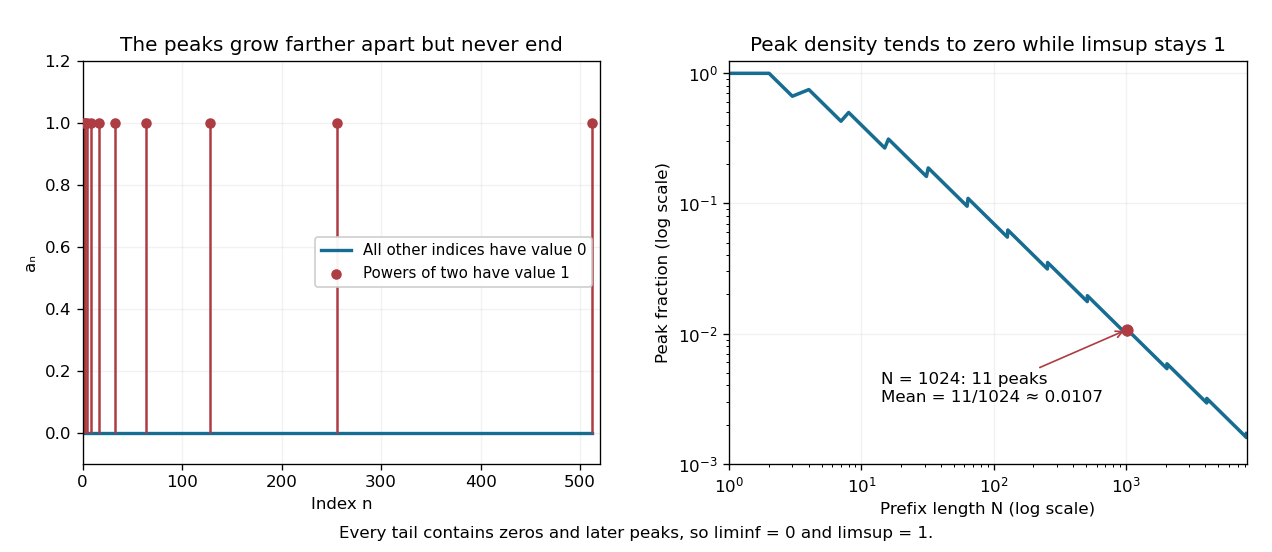
Define a sequence by when is a power of two, including , and otherwise. Every tail of a sequence contains both a later power of two and a later nonpower. Therefore and , and the sequence does not converge. Its peak indices become increasingly sparse, yet never stop appearing.
Through index , the number of peaks is , so their fraction isThe set of powers of two has natural density zero. The same fraction is the Cesàro mean of the first terms, which tends to zero even though the limit superior stays one. At , eleven peaks give mean . An average and a long-run upper edge answer different questions about the same sequence.

A full and faithful functor reflects every existing shape of categorical limit. If the image of a cone is limiting, apply its universal property to the image of any competing cone. Fullness lifts the unique mediating morphism; faithfulness proves the cone equations and uniqueness of the lift. No essential-surjectivity hypothesis is needed.
If has finite categorical limits, every functor preserving pullbacks in a category also preserves equalizers, even when it does not preserve a terminal object. Factor it through the slice category by sending to . This lifted functor preserves pullbacks because the slice forgetful functor reflects them; it also preserves the terminal object, so it preserves finite limits. The slice forgetful functor preserves equalizers, completing the proof.
For a real sequence with no zero terms, the displayed equivalence follows directly by comparing with . Escape to positive infinity implies reciprocal convergence to zero, but the converse does not retain the sign: is a counterexample. If , eventually , and . This proves reciprocal convergence at a nonzero finite limit of a sequence.
Solar limb-darkening drift-scan experiment 2026-10-14
A motivating measurement used the McMath solar optical telescope at Kitt Peak. The Sun's image drifted across a -high, -wide optical slit; a double-pass spectrograph selected wavelength intervals from wide at to at . An EMI 9750 QB photodetector or silicon photodiode supplied a digitized signal: samples were summed into 4096 positions per crossing, including dark and off-limb sky readings. [ref]
Solar limb darkening 1986–1990 (λλ303 to 1099 nm) by Heinz Neckel and Dietrich Labs. §2, p. 93, instrumental compilation: slit dimensions, double pass, detectors, sampling and drift-curve layout; p. 113, acknowledgements identifying the telescope
Controls included daily realignment of optical telescope mirrors, wavelength settings between spectral lines insensitive to the rotational Doppler shift, selection of detectors without detectable hysteresis, and measured electronic nonlinearity corrections below of maximum signal. Limb-position calibration combined centres of gravity of the edge derivative profiles with almanac semidiameters; the preliminary edge shifts were consistent with astronomical seeing of approximately arcseconds full width at half maximum. [ref]
The decreasing centre-to-limb readout gives a specific intensity profile, constraining stratification of the photosphere under a radiative transfer model. Astronomical seeing, instrumental scattering of light, and solar granulation limit this inference; brightness alone does not uniquely determine temperature versus geometric height. These observations need not follow the stipulated linear limb-darkening law.
Small-planet transit weighting 2026-10-14
A dark, opaque circular planet of radius blocks specific intensity over its overlap with the projected star. With and no transit dilution, the instantaneous exoplanet transit depth is exactlyWhen , the entire planetary disk is inside the stellar disk, and specific intensity varies little across that disk, small-planet transit weighting reduces toHere is the projected centre separation divided by . The numerator samples the local specific intensity; the denominator normalizes by the whole star's mean specific intensity. The small-size argument and the distinction between full overlap and ingress are explicit in the original analytic treatment. [ref]
Analytic Light Curves for Planetary Transit Searches by Kaisey Mandel and Eric Agol. §2, p. L171, geometry; §5, p. L174, small-planet approximation restricted to the interior
For a short approximately straight crossing at constant transverse velocity , write with at mid-transit, and let be the transit impact parameter. Then and . With stipulated and , a central crossing has mid-transit exoplanet transit depth approximately , whereas gives . A uniform disk would give for either fully overlapping crossing. The brighter central chord produces a deeper dip and the off-centre chord a shorter crossing at the same .
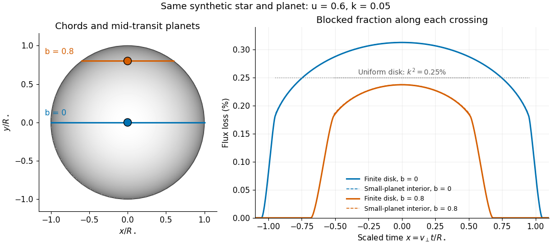
Two transit chords across the same synthetic limb-darkened disk flux distribution
. Stipulated and ; the coloured curves integrate the occulted specific intensity over the finite planetary disk, including ingress and egress. Dashed curves show small-planet transit weighting only where the whole planetary disk is inside the star. Horizontal dotted segments give the uniform-disk full-overlap depth . The chord panel shows mid-transit positions; the horizontal coordinate in the light curve is distance travelled divided by stellar radius, equivalent to scaled time at constant transverse velocity. Details.
At fixed away from the edge, a two-dimensional Taylor's theorem expansion over the symmetric planetary disk cancels the first derivatives; the first correction to the blocked radiant flux is of order if the second derivatives remain bounded. This error estimate is not uniform at the edge, where the radial derivative of the linear limb-darkening law diverges. Ingress, egress, a grazing exoplanet transit, and a crossing of a starspot require the overlap integral or a suitable more complete model. Inferring without the local-to-mean specific intensity ratio can bias the estimated planet radius.
Limb-darkened disk flux 2026-10-14
For a circular stellar disk whose specific intensity is independent of azimuth, its mean specific intensity over projected area isThe polar coordinates element is after angular integration, and . Substitution of the linear limb-darkening law givesFor a distant observer at distance receiving light normally to the detecting plane, the observed radiative flux isIt is spectral irradiance, with units when is per hertz. The local outward radiative flux per actual surface area is instead , a spectral radiant exitance. In a spherical model with the same stellar atmosphere everywhere, the luminosity is and , consistent with the inverse-square law. Compare disks at fixed or fixed total observed radiative flux explicitly: increasing lowers the total in the first comparison, while the second requires a larger .
Linear limb-darkening law 2026-10-14
The linear limb-darkening law parametrizes angular specific intensity by a stipulated limb-darkening coefficient :Here denotes specific intensity at one frequency, or radiance integrated over a specified interval of frequency or wavelength; it does not denote radiant intensity. Within this stipulated range, gives a uniform disk and . The linear limb-darkening law is linear in , while its radial profile is curved. In the linear source function example above, when and .
For the illustrative choice , the specific intensity at , , and the limiting edge is respectively , , and . These are synthetic values, not measurements of the Sun. Real optical spectra and stellar atmospheres need not obey a linear limb-darkening law; more flexible profiles can be necessary for accurate exoplanet transit photometry. [ref]
Analytic Light Curves for Planetary Transit Searches by Kaisey Mandel and Eric Agol. §1, p. L171: the linear law is insufficient for the cited high-quality transit observations; §4 defines a quadratic law
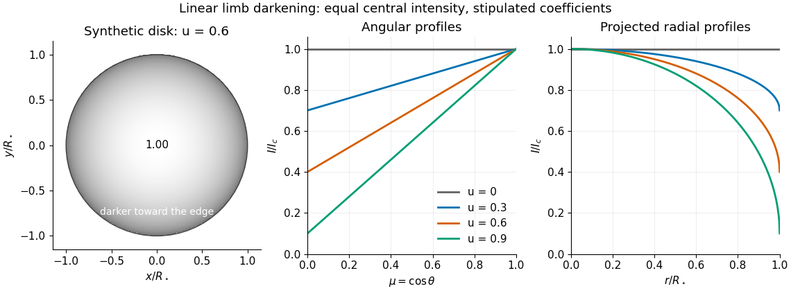
Synthetic stellar disk and angular and radial limb darkening profiles
. The disk uses the stipulated linear limb-darkening law with . The profiles compare four stipulated limb-darkening coefficients at equal central specific intensity. Shading represents relative brightness, without prescribing a wavelength or copying a solar measurement. Details.
For independent unit-variance Gaussian samples with means , testing against unrestricted means gives . The unrestricted maximum-likelihood estimators are the two sample means, while the null estimators are and zero. Under the null, write , , and , with independent standard Gaussian variables. Then decreases pointwise with , so the largest rejection probability occurs at the boundary . There its law is the chi-bar-squared distribution . The exact size- threshold is therefore determined by .
For independent samples from normal distributions with separate unknown means, test equal variances against . Profiling the means gives sample means. Under the null the variance maximum is ; the separate maxima are and . If the latter obey the proposed order, their likelihood quotient isIt decreases strictly as increases. Otherwise the ordered alternative maximum lies on the equal-variance boundary and the quotient is one. Under the null, Cochran's theorem gives independent chi-squared residual sums with degrees , so rejection is in the upper tail of the displayed F-distribution statistic, calibrated at the desired significance level.
For independent multivariate normal observations with unrestricted mean and positive-definite sample covariance matrix , the unrestricted maximum-likelihood estimates are . Requiring a diagonal population covariance matrix gives the same mean and covariance estimate . Both fitted quadratic terms equal , so their likelihood quotient is , where is the sample correlation matrix. Small determinants give evidence against diagonality. For two variables this is a two-sided test of their sample correlation.
For independent observations from a nonsingular multivariate normal distribution with unknown mean, let . The unrestricted maximum-likelihood estimator of covariance is , while the diagonal restriction gives . The fitted trace terms both equal , so twice the log-likelihood difference is , where is the sample correlation matrix. Under the diagonal null hypothesis and fixed dimension, the Wilks theorem gives .
Closed-subgroup theorem 2026-10-14
Every closed subgroup of a finite-dimensional Lie group is an embedded submanifold and a Lie subgroup. Closedness alone forces the compatible smooth structure; smoothness need not be assumed in advance. The proof constructs the Lie algebra of a closed subgroup from one-parameter subgroups, then uses local product coordinates for a closed subgroup.
A Lie group homomorphism intertwines one-parameter subgroups and therefore obeys the displayed identity. A connected Lie group is generated by an identity neighbourhood in an exponential chart, so its homomorphism is uniquely determined by the differential at the identity. On a disconnected group, only the restriction to its identity component is determined this way; the images of the other components require extra data.
Lie group isomorphism 2026-10-14
An isomorphism of Lie groups is a group isomorphism that is also a diffeomorphism. Both the homomorphism and its inverse preserve the smooth structures. Its identity differential is a Lie algebra isomorphism, but an isomorphism of Lie algebras determines a global Lie group isomorphism without extra period data only for connected simply connected groups.
Proper Lie group action 2026-10-14
A Lie group action on is proper if from to is a proper map. A free proper smooth action has a smooth quotient manifold, with the quotient map a submersion and principal bundle. Proper actions with stabilizers can have orbit-type strata and singular quotients. These qualifications are necessary before treating an orbit space as a smooth phase space.
Alternating Lie bracket 2026-10-14
A Lie bracket is alternating when for every . This condition is imposed in every characteristic of a field. Bilinearity gives , hence antisymmetry of a Lie bracket. Requiring alternation directly keeps the definition correct in characteristic two.
Matrix commutator from a logarithm chart 2026-10-14
If the matrix logarithm identifies a neighborhood of the identity in a Matrix Lie group with a neighborhood of zero in its tangent subspace, the logarithm of the displayed group commutator belongs to that subspace. Divide it by and take the limit. Finite-dimensional linear subspaces are closed, proving closure under the matrix commutator without attempting to give a nonsmooth square-root reparametrization a velocity.
Integration of a Lie algebra homomorphism 2026-10-14
For a connected simply connected source Lie group, every Lie algebra homomorphism integrates uniquely to a Lie group homomorphism. Along a path from the identity, transport its left logarithmic velocity by and solve the corresponding left-invariant differential equation in the target. The Maurer-Cartan equation and preservation of brackets make the endpoint invariant under fixed-endpoint homotopies. Simple connectedness removes path dependence, and path concatenation proves multiplicativity.
There are unlisted articles, also show them or only show them.