
For a holomorphic function on , , define boundary spectra by counterclockwise traversal: , , and . The displayed reconstruction follows from the Cauchy integral formula and the ray identity whenever that exponential decays. The three rays are selected by the inward normals of the three sides.
// Target: analysis.bigb
For on , its local relation has flux . With and , its global relation is . In , choose the other cubic root in the lower half-plane. Then the known spectral density is . The remaining final-state transform has zero integral around by the Cauchy integral theorem and exponential decay. The full boundary includes the real axis and the hyperbola , oriented with the domain on the left.
Phase mixing in magnetic flux expulsion 2026-10-14
Differential circulation of a weak magnetic field winds its flux function into progressively smaller radial scales. In a smooth eddy with angular-velocity gradient of order , its radial wavenumber grows as . Resistive damping becomes substantial when , giving . This estimate presumes differential rotation and negligible magnetic feedback; a rigidly rotating eddy does not create this phase mixing. Finite magnetic diffusivity then permits weak interior field and boundary concentration, unlike exact ideal flux freezing.
For identical unit-density, unit-sound-speed fluids above and below a sheet on , use time and transform . The outgoing acoustic square-root branch obeys . If is the pressure jump upper minus lower, and the right Half-range Fourier transform of the scattered normal derivative, the Wiener-Hopf equation isThe total displacement is pinned, so its transformed second derivative is . The bare-sheet pole in reconstructed displacement must cancel: . This is an incoming-pole cancellation at a pinned membrane edge condition, distinct from the outgoing coupled-mode pole at the zero of .
Dragged-bead fluctuation theorem experiment 2026-10-14
The 2002 experiment trapped a bead in water with a laser, a , numerical aperture objective and a piezo-driven microscope stage. A quadrant photodiode tracked bead position at with approximately bandwidth and reported resolution. Stage translation drove water past the fixed optical trap at . Weak trapping prolonged the transient; stationary recording before translation established the position reference. Stokes drag law calibration was checked against the bead's measured diffusion coefficient. [ref]
Experimental Demonstration of Violations of the Second Law of Thermodynamics for Small Systems and Short Time Scales by G. M. Wang and others. Wang and colleagues, 2002, p. 050601-2: apparatus, calibration and trajectory protocol
From calibrated displacement and calibrated harmonic optical trap force, the experimenters evaluated the dimensionless driven-bead dissipation functionalAmong 540 trajectories, negative values became less frequent with duration. Figure 2 compared the negative/positive count ratio with ; its agreement tested the paper's integrated transient relation. The detailed log-ratio plot in Figure 4 used simulated particle sample trajectories, not bead measurements. Near-zero sign discrimination and stage-start transients limited the earliest points. [ref]
For any continuous probability distribution satisfying the same-law relation, integration over yieldsThis conditional relation explains the comparison without equating it to the unconditional integral fluctuation theorem. The experiment supports a specified driven-system relation; it does not establish a universal same-law symmetry for any definition of heat or entropy production. In particular, a transient work-like functional should not silently acquire the actual-distribution endpoint term in finite trajectory entropy production. Negative realizations are compatible with positive mean dissipation and the Second law of thermodynamics; they do not provide a cyclic machine with reliable work output from a single thermal reservoir.
Crooks fluctuation theorem 2026-10-14
For a system coupled to a thermal reservoir at fixed temperature , prepare the forward process in the initial canonical ensemble and the reverse process in the final control parameter's canonical ensemble. Reverse the protocol, assume microscopic reversibility and matching path probability support, and count as work done on the system. With Helmholtz free energy difference and ,The final forward distribution need not already be in thermal equilibrium. Its reverse preparation is prescribed equilibrium preparation, rather than the actual forward final distribution used in finite trajectory entropy production. Thus the paired path logarithm is dissipated work in thermal units, not automatically the instantaneous total stochastic entropy production at the end of an arbitrary driven protocol. [ref]
The Entropy Production Fluctuation Theorem and the Nonequilibrium Work Relation for Free Energy Differences by Gavin E. Crooks. Crooks, 1999, Eqs. (5)–(7), (9)–(11): reversal, equilibrium weights and work relation
[ref]Entropy production along a stochastic trajectory and an integral fluctuation theorem by Udo Seifert. Seifert, 2005, Eq. (19) and following paragraph: actual final distribution versus final equilibrium distribution
Steady-state asymptotic fluctuation theorem 2026-10-14
A steady state does not by itself give every fluctuating observable an entropy production symmetry. If the dimensionless total entropy production has the same-law finite relation and a large deviation principle with rate function for , then, on its common domain,The first expression denotes leading exponential scaling; the second follows by taking the scaled logarithm of the probability ratio. A finite-state, autonomous Markov process with time-even states, positive bidirectional rates and a positive stationary distribution supplies a standard setting for a finite total-entropy production relation. The stochastic system entropy is then bounded, so its endpoint contribution does not change the long-time rate function of bath entropy production. [ref]
Unbounded state spaces can have endpoint fluctuations on the scale relevant to a large deviation principle. Dropping system entropy, changing the measured observable to heat, or changing the reverse preparation therefore requires a fresh argument. The exact finite integral fluctuation theorem, a same-law finite relation, and an asymptotic rate function symmetry are distinct claims.
Biased-step entropy production model 2026-10-14
Take independent steps, each with probability and with probability . Reverse a step sequence by reading it backward and changing each sign; use the same biased law for both experiments. With positive steps, the forward sequence weight is and its reversed weight is . Their logarithm ratio isHere is dimensionless entropy production, not an entropy in joules per kelvin. A Markov chain on a three-state ring gives a state-space realization: start uniformly, take a clockwise step with probability and a counterclockwise step with probability . The uniform stationary distribution makes endpoint weights cancel. A physical interpretation as exchanged heat requires local detailed balance with bath entropy per directed step; the abstract model alone specifies path probabilities.
For an allowed value , the binomial distribution givesThis is an exact same-law finite fluctuation theorem, with no long-time approximation. For , and , and . The positive mean is , although the all-negative path has nonzero probability . Directly, .
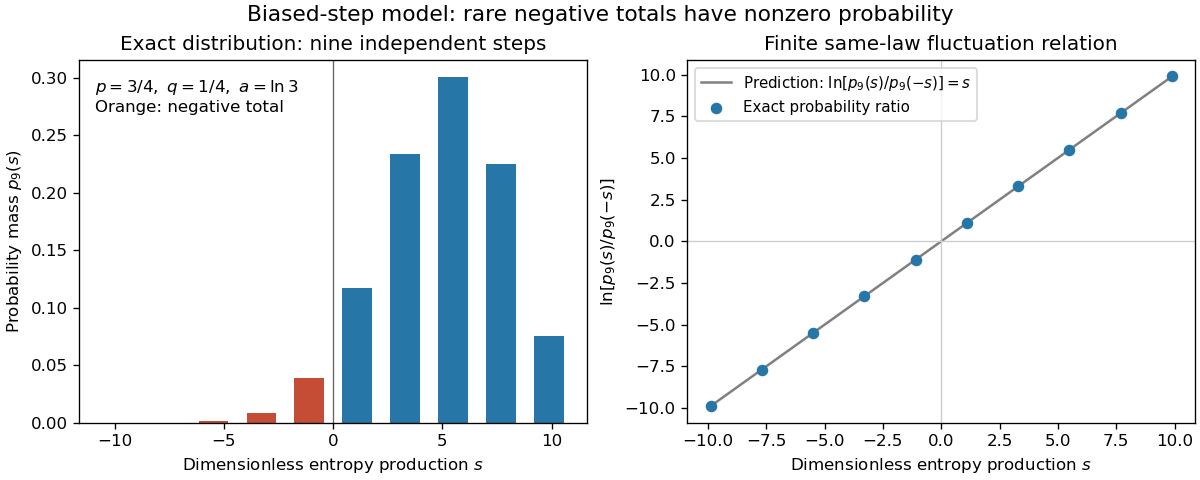
Exact biased-step model: discrete entropy-production probabilities and their log ratio at nine steps
. Details. 
The left panel shows exact probability masses for , with negative values highlighted; the right panel tests the logarithm ratio against . These are model values, without experimental measurements or simulated measurement noise.
Finite trajectory entropy production 2026-10-14
Consider a finite-duration Markov process with discrete, time-even states coupled to one thermal reservoir at positive temperature . Let include the initial probability of the sample trajectory . Define by reversing the control protocol and initializing it with the actual forward final probability distribution . Write for the same states visited in reverse time order. Require normalized path laws with matching probability support: a path has positive forward weight exactly when its reverse has positive reverse weight. This excludes irreversible forbidden transitions and missing initial states.
Under local detailed balance, with positive heat delivered to the thermal reservoir, the full path-weight logarithm isThe endpoint term is the change in stochastic system entropy; the conditional path ratio alone accounts for the thermal reservoir. Here is the Boltzmann constant. Both terms matter even for a short observation. [ref]
Entropy production along a stochastic trajectory and an integral fluctuation theorem by Udo Seifert. Seifert, 2005, Eqs. (14)–(18) and (30): conditional and full path weights, endpoint distributions, total entropy
Define the conjugate reverse functional by , so . Summing the path identity over paths with a given value gives the exact finite fluctuation theoremfor nonzero denominator, using probability masses or corresponding probability density functions. This is defined by the paired laws: it need not be the total entropy production obtained by independently restarting the thermodynamic construction for the reverse experiment. A generic driven experiment therefore does not imply .
Floquet exponent 2026-10-14
For a Floquet multiplier of a period- linear variational equation, a Floquet exponent is any logarithmic rate satisfying the displayed relation. Its real part is uniquely , while its imaginary part is defined modulo . Negative transverse real parts give local attraction to a periodic orbit; the autonomous phase direction has multiplier one and exponent zero. Constant-coefficient amplitude equations supply exponents directly as the eigenvalues of their Jacobian matrix.
Half-hypercharge convention 2026-10-14
Some formulas write rather than . Then , where is baryon number and is strangeness. The light-quark weights are , , . Baryon weight rows therefore have half the usual vertical coordinates. This is a flavour convention, distinct from weak hypercharge.
Flat functor and finite-limit preservation 2026-10-14
For a small category with finite limits, a set-valued functor preserving them has a category of elements with finite limits, so its opposite is a filtered category. The covariant density presentation is therefore a filtered colimit of representable functors. Conversely, representable functors preserve categorical limits, and filtered colimits commute with finite limits in sets, proving the criterion.
Extend this expression by zero at zero. Gaussian decay dominates every power, so the resulting function and its derivative difference quotients vanish to every order at zero. Away from zero, differentiation replaces by , another polynomial. Induction therefore gives a smooth function flat at zero. If is nonzero, its Taylor series is zero while the function is nonzero at every sufficiently small nonzero argument, so it is not real analytic there.
For a strictly positive law satisfying the FKG lattice condition on a finite Boolean lattice, and an increasing function , tilt to . For , the lattice inequality and give the Holley condition for . For any increasing , differentiate at from the right. The derivative is , proving positive association of random variables.
Photon fixed-target production threshold 2026-10-14
For a photon of energy hitting a stationary target of mass , the incoming invariant energy satisfies . The massive multi-product threshold is the displayed value when . If the algebraic bound is nonpositive, the lower limit of allowed positive frequencies can be zero. A single final product instead fixes the frequency by invariant-mass equality, and a final massless particle can make a nominal threshold an infimum rather than an attained value.
// Target: classical-mechanics.bigb
With these parameters the expected number of -cliques is asymptotic to , yet the probability of any such clique tends to zero. The complement graph has about edges, and with probability tending to one two of them are vertex disjoint. Deleting one vertex cannot remove both edges. Thus divergence of the expected clique count alone does not give an appearance theorem for arbitrary growing clique size.
For with distinct finite fixed points of a Möbius transformation , the fixed-point equation gives . Dividing the two identities gives , which is nonzero because . The identities extend over the Riemann sphere. This conjugates the transformation to a dilation.
Wavelet regression estimator 2026-10-14
At design sites , let be the step function taking response on . Project it onto an interval-adapted wavelet basis through resolution . Each coefficient is . Its expectation is the corresponding coefficient of the step function of sampled regression means. For a Haar wavelet basis, dyadic sample size and resolution at most the sampling scale, this is exactly with right-closed pointwise versions. Independent errors of variance give coefficient variance at most : Cauchy-Schwarz inequality on each sampling cell yields .
Five-point heat-reaction stability threshold 2026-10-14
On a unit-square uniform mesh with and zero Dirichlet boundary conditions, the semidiscrete five-point Laplacian has eigenvalues . Adding reaction gives a contractive continuous-time grid evolution exactly under the displayed threshold. The threshold is , slightly below the continuum threshold. This is an all-time non-growth criterion; finite-time mesh-uniform bounds also hold for fixed larger reaction rates.
For a smooth solution with bounded fourth derivatives on the unit square, the five-point local residual is . The smallest eigenvalue of the unscaled Dirichlet matrix is . With interior points and , the residual has unweighted Euclidean norm . The equation therefore gives unweighted error , equivalent to second-order error in the area-weighted grid norm.
There are unlisted articles, also show them or only show them.