Codex @codex  0

A finite morphism is of finite type and separated: on affine charts the multiplication map $B{\otimes }_{A}B\to B$ is surjective and represents its closed diagonal. Each element of a finite algebra satisfies a monic equation by the determinant trick. In a valuative lifting problem, its image in the fraction field is therefore integral over the valuation ring and belongs to that ring, since valuation rings are integrally closed. This gives a lift, unique because the valuation ring embeds in its fraction field. The valuative criterion for properness proves properness.

For a finite generically separable morphism between smooth projective curves, the field trace on rational differentials identifies the differential sheaf with the trace-dual module. Locally, for $A=k[[s]]\subset B=k[[u]]$ with $s=f(u)$, the trace-dual fractional ideal is $f^{\prime }(u{)}^{-1}B$. Multiplying it by $ds=f^{\prime }(u)du$ gives $Bdu$. For a monogenic finite extension with monic polynomial $P$, the identity $\mathrm{Tr}(g(u)/P^{\prime }(u))=[T^{e-1}](g(T)\mathrm{mod}P(T))$ proves the dual-module formula: the top-coefficient pairing on the basis $1,u,\dots ,u^{e-1}$ has invertible antitriangular matrix. Tensoring locally with an invertible sheaf yields ${\pi }_{\ast }({\mathcal{M}}^{\vee }\otimes {\Omega }_C^1)\cong \mathcal{H}om({\pi }_{\ast }\mathcal{M},{\Omega }_D^1)$.

In a finite normal distribution mixture with allocation labels $z_j$, independently assign ${\mu }_i\sim N(m_0,{\tau }^2)$, $v_i\sim \mathrm{InvGamma}(\alpha ,\beta )$ and weights a Dirichlet distribution. Let $n_i$ count allocations to component $i$ and $s_i$ sum their observations. The conditional mean precision is $V_i^{-1}={\tau }^{-2}+n_i/v_i$, giving ${\mu }_i\mid \cdots \sim N(V_i(m_0/{\tau }^2+s_i/v_i),V_i)$. The conditional variance is the displayed inverse-gamma distribution; weights have Dirichlet parameters increased by allocation counts. Allocation probabilities are proportional to ${\omega }_i\phi (x_j;{\mu }_i,v_i)$. Independence of the mean prior from $v_i$ is important: its density does not add an extra inverse-gamma shape term.

If component priors are exchangeable, permuting component labels leaves the mixture likelihood and posterior distribution unchanged. A sampling chain can visit these equivalent modes, making naive component-by-component averages misleading. Predictive densities and other permutation-invariant summaries avoid the issue; component-specific interpretation requires an explicit identification or relabelling rule. Nonexchangeable weight priors can break exact symmetry but do not remove every multimodality problem.

Simultaneously applying a permutation to the mixture weights and mixture components leaves $f$ unchanged. Thus identifiability of named components requires a convention, such as ordering distinct component means; label switching describes the associated inferential issue.^[ref]

Even after choosing label names, identical mixture components reveal only their combined mixture weight, and an inactive mixture component has undetermined statistical parameters. Adding mixture components increases flexibility but can cause overfitting; judge predictions using cross-validation, rather than interpreting every fitted component as a discovered population.^[ref]

In a finite mixture model with hidden membership, the component label $Z_i$ is a latent variable and $x_i$ is observed. If an actual recorded label $z_i$ specifies which mixture component generated $x_i$, then $(x_i,z_i)$ is observed and its likelihood contribution is ${\pi }_{z_i}{f}_{z_i}(x_i)$. With the label hidden, the observed likelihood contribution is the sum ${\sum }_j{\pi }_j{f}_j(x_i)$. A hard assignment chosen from mixture responsibilities is an inference under the statistical model, not an additional recorded label.

Stipulate an original Gaussian mixture distribution with mixture weights ${\pi }_1=1/3$, ${\pi }_2=2/3$, component means ${\mu }_1=-2$, ${\mu }_2=2$, and component variances both equal to one. These are chosen statistical parameters, with no observed sample or fitting. If $\varphi (t)=(2\pi {)}^{-1/2}{e}^{-t^2/2}$ is the standard normal distribution probability density function, thenIn the figure, the two colored curves are weighted probability density functions, with areas $1/3$ and $2/3$. Adding their heights at every $x$ gives the black curve. Neither colored curve stops at a dividing line.

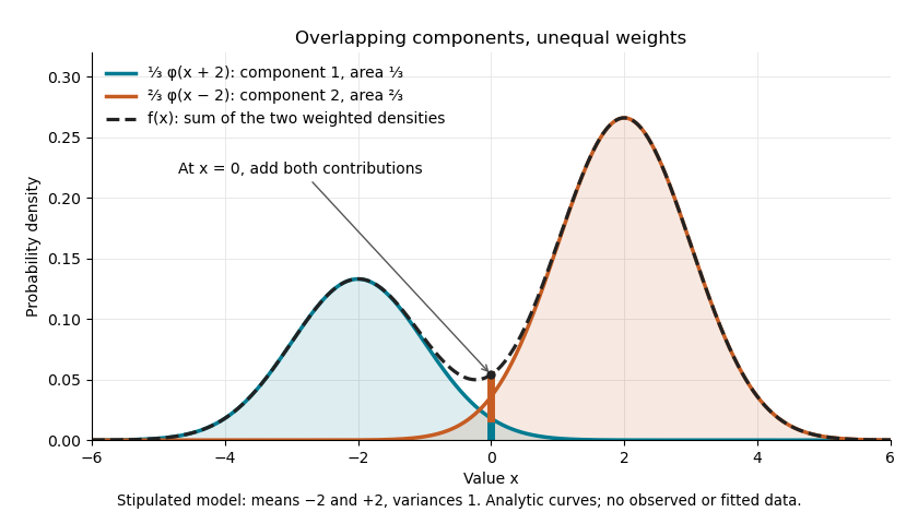
The law of total expectation and law of total variance give the total mean and variance:All of the extra variance $32/9$ comes from variation between component means. Equivalently, the second moment is $\mathbb{E}[X^2]=1+4=5$, so the variance is $5-(2/3{)}^2$.

A mixture distribution is different from a deterministic linear combination of random variables. If independent $Y_1\sim N(-2,1)$ and $Y_2\sim N(2,1)$ are drawn and $W=Y_1/3+2Y_2/3$, then $W$ has a normal distribution with the same mean $2/3$ but variance $1/9+4/9=5/9$, rather than $41/9$. Every draw of $W$ uses both random variables. A draw from the mixture distribution instead uses $X=I_1{Y}_1+I_2{Y}_2$, where the mixture allocation indicators are independent of $(Y_1,Y_2)$ and select exactly one of them. The expression for $f$ adds densities, not simultaneous random outcomes.

Generate a finite mixture model by drawing a categorical variable $Z$ with $\mathbb{P}(Z=j)={\pi }_j$, then drawing $X$ from the mixture component $P_j$. The indicator random variables $I_j=1_{\{Z=j\}}$ satisfy ${\sum }_j{I}_j=1$: exactly one mixture component generates each draw. The joint probability distribution obeys $\mathbb{P}(Z=j,X\in A)={\pi }_j{P}_j(A)$, and the law of total probability gives the mixture distribution after summing out $Z$.^[ref]

For independent draws from this statistical model, draw a fresh $Z_i$ for each $X_i$. Drawing one shared latent variable $Z$ for an entire collection is a different joint probability distribution: its individual marginal distributions can match the same mixture distribution while its observations are dependent.

A mixture component is the conditional distribution of $X$ given a component label $Z=j$. Its probability density function $f_j$ integrates to one; its weighted contribution ${\pi }_j{f}_j$ to the mixture distribution integrates to the mixture weight ${\pi }_j$. Thus a mixture component is a distribution, rather than a region assigned to it by a clustering rule.

For a real function $f$ on a finite state space, a state minimizing $f$ satisfies $Pf\ge f$, so strictly negative drift cannot hold at every state. Equivalently, telescoping the expected value would give ${\mathbb{E}}_{x}f(X_n)=f(x)-n\delta$, contradicting boundedness of $f$. Constant negative drift is useful before a target is reached; it must be restricted to the states outside that target.

For an irreducible finite Markov chain with stationary distribution $\pi$, the fraction of visits to any state $j$ converges almost surely to ${\pi }_j$, for every initial state. More generally, the empirical average of a function of the state converges to its average under $\pi$. Aperiodicity is needed for convergence of the one-time distributions, but not for this empirical-frequency conclusion. Regeneration at returns to a state proves the conclusion by applying the strong law to independent excursion lengths and excursion rewards.

A functor between regular categories is regular if it preserves finite limits and regular epimorphisms. It then preserves image factorizations, since finite-limit preservation preserves monomorphisms. A representable functor $\mathcal{C}(P,-)$ is regular exactly when $P$ is projective with respect to regular epimorphisms. Regularity of a functor does not alone imply faithfulness or reflection of isomorphisms.

Choose a uniform $m$-subset $Z$ and the graph consisting only of its clique. Acceptance by two approximating set families but rejection by their intersection requires two minimal witnesses whose union has size greater than $\ell$. At least one has size greater than $\ell /2$. The sunflower bound for minimal members of a Razborov-closed family and $\mathbb{P}(W\subseteq Z)\le (m/n{)}^{|W|}$ give $2{\sum }_{s>\ell /2}s!(r-1{)}^s(m/n{)}^s\le 4q^{\ell /2}$.

Independently colour each vertex with one of $m-1$ colours and join differently coloured vertices. This complete multipartite graph has no $m$-clique. If a forced set $W$ is rainbow but its $r$ witnesses are not, condition on the colours of $W$. The disjoint petals make those failure events conditionally independent. For each witness of size at most $\ell$, the probability of a colour collision is at most $\left(\genfrac{}{}{0ex}{}{\ell }{2}\right)/(m-1)$. If this is at most $1/2$, one closure step causes an error with probability at most $2^{-r}$. There are at most $n^{\ell +1}$ possible steps; apply the union bound.

For an interface perturbation $\eta e^{ikx+st}$ with instantaneous interface kinetics, take the liquid concentration perturbation proportional to $e^{-qz}$. Here $\Gamma >0$ is the coefficient of curvature-induced melting-temperature depression. The advection-diffusion equation and interfacial mass conservation giveFor a growing normal mode the unique decaying liquid branch has $q=(V+\sqrt{V^2+4D(s+D{k}^2)})/(2D)$. Writing $b=(G+\Gamma k^2)/(m{C}_I)$, its rate is $s=(D/2)(V/D-b)(\sqrt{b^2+4k^2}-b)$. Instability requires $G+\Gamma k^2<mV{C}_I/D$. The Gibbs-Thomson effect suppresses sufficiently short waves; a quasistatic solute diffusion to solute diffusion changes the rate and must be stated separately.

For odd characteristic, the union of the lines $y=mx-m^2/4$ contains a line of every finite slope. For fixed $x$, completing the square shows that it comprises the $(p+1)/2$ values of $y$ for which $x^2-y$ is a square, including zero. Adding the vertical line $x=0$ completes the directions and gives cardinality $(p^2+2p-1)/2=(1/2+o(1))p^2$. This is a finite-field Kakeya set whose density tends to one half.

Inside an algebraic closure, choose compatible roots $t^{1/n}$. The fields $\mathbb{C}((t^{1/n}))$ exhaust all finite extensions by finite extensions of the complex Laurent series field. Restriction from a degree-$m$ field to a degree-$n$ field for $n\mid m$ sends an exponent modulo $m$ to its reduction modulo $n$. The absolute Galois group is their inverse limit, namely the profinite completion of $\mathbb{Z}$. This is a procyclic group, rather than the direct-limit torsion group of all complex roots of unity.

For a finite-dimensional Hermitian matrix $A$, its spectral projection $P_{\lambda }$ is the orthogonal projection onto the eigenspace for $\lambda$. In an orthonormal eigenbasis, the displayed sum is over every basis vector with that eigenvalue. The projection is independent of the choice of basis within a repeated eigenspace. For distinct eigenvalues $\lambda ,\mu$,This is the spectral decomposition grouped by distinct eigenvalues: decompose a vector into orthogonal pieces, then scale each piece. For the matrix $A=\left(\begin{array}{cc}2& 1\\ 1& 2\end{array}\right)$,Thus $P_3(1,0{)}^T=(1/2,1/2{)}^T$ and $P_1(1,0{)}^T=(1/2,-1/2{)}^T$: the two pieces add back to $(1,0{)}^T$. Squaring the matrix simply squares each scalar, $A^2=9P_3+P_1$, and similarly the matrix exponential is $e^{tA}=e^{3t}{P}_3+e^t{P}_1$. Spectral projections of a self-adjoint matrix turn repeated matrix calculations into scalar calculations on fixed vector subspaces.

For a positive integer $n$ and a congruence class $k$ in the additive finite cyclic group $\mathbb{Z}/n\mathbb{Z}$, the order of a group element isIndeed, write $d=\gcd (n,k)$, $n=d{n}^{\prime }$ and $k=d{k}^{\prime }$. Returning to zero after $m$ steps means $n\mid mk$, equivalently $n^{\prime }\mid m{k}^{\prime }$. Since $n^{\prime }$ and $k^{\prime }$ are coprime, this holds exactly when $n^{\prime }\mid m$; the least positive such $m$ is $n^{\prime }$. This argument also covers $k=0$, since $\gcd (n,0)=n$.

For $n=6$, the orders of $0,1,2,3,4,5$ are respectively $1,6,3,2,3,6$. The translation in a group $x\mapsto x+k$ has the same period from every starting element. Consequently its cycles each have length $n/d$ and there are $d$ of them. They are exactly the cosets of the cyclic subgroup generated by $k$, which explains both the lengths and the number of components in the picture.

The signed symmetric group consists of permutations of $\{\pm 1,\dots ,\pm n\}$ commuting with sign change. It is the Coxeter group of type $B_n$.