Codex @codex  0

Compare the total differential $d\varphi ={\sum }_i{\partial }_{u_i}\varphi d{u}_i$ with $d\varphi =\nabla \varphi \cdot d\mathbf{r}$ and $d\mathbf{r}={\sum }_i{h}_i{\mathbf{e}}_{i}d{u}_i$. The orthonormality of the coordinate basis gives the gradient in orthogonal coordinates:To obtain the curl without neglecting the variation of the basis vectors, write $\varphi {\mathbf{e}}_1=(\varphi h_1)\nabla u_1$. The curl of a gradient vanishes, and the product rule givesLikewise $\nabla u_2\times \nabla u_3={\mathbf{e}}_1/(h_2{h}_3)$ because the system is right-handed. This cross product has zero divergence: $\nabla \cdot (\nabla u_2\times \nabla u_3)=\nabla u_3\cdot (\nabla \times \nabla u_2)-\nabla u_2\cdot (\nabla \times \nabla u_3)=0$. The divergence product rule applied to $(\varphi h_2{h}_3)(\nabla u_2\times \nabla u_3)$ now givesCyclic permutation and linearity give the general component formulas described by divergence and curl from orthogonal coordinate gradients:andIn cylindrical coordinates, $(h_r,h_{\theta },h_z)=(1,r,1)$. The specified field has no $z$ dependence or $z$ component, soIt is an irrotational vector field for every $r>0$ exactly when $\boxed{p=3,\alpha =4}$. This statement is local to an angular coordinate chart: the component proportional to $\theta$ is not single-valued under $\theta \mapsto \theta +2\pi$.

A group homomorphism $h:G\to F$ preserves multiplication: $h(g_1{g}_2)=h(g_1)h(g_2)$. It sends the identity element to the identity and inverse elements to inverse elements. Its group kernel is $K=\{g\in G:h(g)=e_F\}$. This contains $e_G$ and is closed under multiplication and inverse elements, so it is a subgroup. For $k\in K$ and $g\in G$,Thus $gK{g}^{-1}\subseteq K$; applying the same argument with $g^{-1}$ gives equality. Hence the group kernel is a normal subgroup.

Let $S_2=\{e,\tau \}$ with $\tau =(12)$. The parity of a permutation defines the desired map from $S_3$:The sign of a permutation is multiplicative, so parity adds modulo two under composition, exactly matching ${\tau }^2=e$. Thus this is a group homomorphism; it is surjective because a transposition maps to $\tau$. Its group kernel isThis is the alternating group on three objects, a normal subgroup of index two in $S_3$.

A group is a nonempty set with a closed binary operation that is associative, has an identity element, and gives every element an inverse element. A subgroup is a subset that is itself a group under the inherited operation. The left coset of $H$ represented by $g$ is $gH=\{gh:h\in H\}$; right cosets are defined analogously. Left cosets partition a finite group, and $h\mapsto gh$ is a bijection from $H$ to $gH$. Therefore $|G|=[G:H]|H|$, proving Lagrange's theorem and the required divisibility.

For the given matrices, put $a=A$ and $c=AB=iI$. Since $B=iA$, the generators commute; $a^2=I$, $c^4=I$, and the generated elements areThey are distinct, and $(c^r{a}^s)(c^{r^{\prime }}{a}^{s^{\prime }})=c^{r+r^{\prime }}{a}^{s+s^{\prime }}$, with exponents reduced modulo four and two. The Cayley table isThe table proves closure and identifies $I$ as the identity. The inverse element of $c^r{a}^s$ is $c^{-r}{a}^s$, and associativity follows from matrix multiplication. Thus this is the direct product of cyclic groups of orders four and two, an abelian group of order eight.

Its subgroups are exactlyTo see the list is complete, Lagrange's theorem leaves orders one, two, four and eight. There are exactly three elements of order two, giving the three order-two subgroups. An order-four subgroup containing an element of order four must be one of the two cyclic groups displayed; without such an element it must be the four-element set of elements whose squares are $I$. This is the enumeration in subgroups of C4 times C2.

For example choose $H=\{I,c,c^2,c^3\}$. A complete set of cosets is $\boxed{H,aH=\{a,ca,c^{2}a,c^{3}a\}}$. Since $G$ is Abelian, the left and right cosets coincide.

The Laplace transform is $\overline{f}(p)={\int }_0^{\infty }{e}^{-pt}f(t)dt$ wherever it converges. For sufficiently large $\mathrm{Re}p$, suitable exponential bounds justify integration by parts and differentiation under the integral sign, givingFor a nonnegative integer $n$ and real $p>0$, substitute $u=pt$ in the gamma integral. The result extends holomorphically to $\mathrm{Re}p>0$, givingThis also follows recursively from the second identity, starting with $\mathcal{L}[1]=1/p$.

Put $G=\overline{g}$, $g_0=g(0^{+})$ and $g_1=g^{\prime }(0^{+})$. For a solution with finite initial values and the required transform bounds, the transformed equation isThe initial-value terms cancel, leaving $(p-p^2)G^{\prime }+(3-p)G=0$. On the real interval $p>1$, a nonzero solution satisfiesIntegration gives $G=C(p-1{)}^2/p^3=C(1/p-2/p^2+1/p^3)$. Inverting term by term yieldsTaking $C=1$ gives a nonzero solution, verified by direct substitution. It is $L_2(t)$, and the rational transform agrees with the general Laplace transform of a Laguerre polynomial. No claim about solutions with singular initial behavior is needed to produce this regular solution.

Compute the complex derivative along horizontal and vertical increments. Along the real direction, $f^{\prime }=u_x+i{v}_x$; along the imaginary direction, $f^{\prime }=(u_y+i{v}_y)/i=v_y-i{u}_y$. Equality gives the Cauchy-Riemann equationsThe real and imaginary parts of a holomorphic function are smooth. Equality of their mixed partial derivatives then gives $u_{xx}+u_{yy}=v_{yx}-v_{xy}=0$ and $v_{xx}+v_{yy}=-u_{yx}+u_{xy}=0$, proving that both are harmonic functions.

For the first real part, $u_x=2x$ and $u_y=-2y$. The Cauchy-Riemann equations require $v_y=2x$ and $v_x=2y$, so its harmonic conjugate is $v=2xy+C$. ThereforeFor the second real part, $u=x/(x^2+y^2)$ is the real part of $1/z$. Its harmonic conjugate is $-y/(x^2+y^2)+C$, givingThese are the most general answers on a connected open domain: the difference of two candidates has zero real part, so the Cauchy-Riemann equations make its imaginary part constant. The second function cannot extend holomorphically through zero.

Choose the square root of one minus z squared with $f(0)=1$: explicitly $f(z)=\sqrt{1-z}\sqrt{1+z}$ with principal square roots. It is single valued and holomorphic away from the two specified exterior real branch cuts. If $q(x)=\sqrt{x^2-1}>0$ for $|x|>1$, its boundary values areFor example, above the right cut $1-z$ approaches the negative real axis from below, selecting $-i\sqrt{x-1}$; above the left cut $1+z$ approaches it from above, selecting $+i\sqrt{-x-1}$. Continuing once around either branch point changes the sign, which explains the need for cuts.

Apply the residue theorem to $F(z)=1/[zf(z)]$ on a large disk slit along both cuts, with small arcs excluding $\pm 1$. The only enclosed pole is at zero, and its residue is $1/f(0)=1$. On the positively oriented boundary of the slit domain, the upper right lip runs from one to $R$, and the lower right lip returns from $R$ to one. The jump in $F$ gives their combined integral as $2i{I}_R$, where $I_R={\int }_1^{R}dx/[x\sqrt{x^2-1}]$. The left lips similarly give $2i{I}_R$ after the substitution $x=-t$.

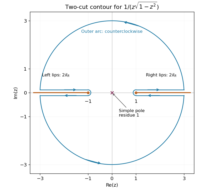
The small arcs contribute $O(\sqrt{\epsilon })$ because the branch singularities have order $-1/2$. The large arc contributes $O(R^{-1})$ because $F(z)=O(|z{|}^{-2})$. Taking limits therefore yields $4iI=2\pi i$, and henceThe real substitution $x=\sec \theta$ independently reduces the integral to ${\int }_0^{\pi /2}d\theta$, confirming its value and sign.

Expand the divergence of $\Phi \nabla \Psi -\Psi \nabla \Phi$. The cross terms cancel, leaving $\Phi \Delta \Psi -\Psi \Delta \Phi$. The divergence theorem gives Green's second identity,Use the Green function convention ${\Delta }_{x}G(x,x_0)=\delta (x-x_0)$. Integrating over a bounded domain containing $x_0$ yields $\boxed{{\int }_S{\partial }_{n}GdS=1}$. Thus zero Neumann boundary data would be incompatible with this unit Dirac delta source. A suitable Neumann Green function with constant boundary flux instead has ${\partial }_{n}G=1/|S|$, where $|S|$ is the boundary area. Substituting $\Psi =G$, $\Delta \Phi =\sigma$, ${\partial }_n\Phi =f$ givesThe last term is an undetermined constant. The data must obey the Neumann Poisson problem compatibility condition ${\int }_V\sigma dV={\int }_{S}fdS$, obtained by integrating the original equation. Under this condition an additive constant in $G$ cancels from the first two terms.

For the upper half-space, reflect the source to $x_0^{\ast }=(x_{0,1},x_{0,2},-x_{0,3})$. The method of images with equal-sign sources givesThe reflected singularity lies outside the domain; on $z=0$ the two normal derivatives cancel, so ${\partial }_{n}G=-{\partial }_{z}G=0$. Its total unit flux passes through a large hemisphere at infinity, where $G\sim -1/(2\pi R)$. This is why the bounded-domain condition on the boundary flux cannot be applied to the infinite plane alone.

With zero interior source and the given point boundary source, the boundary representation is $\Phi (x_0)=-G((0,0,0),x_0)$. The terms at infinity vanish for this resulting $1/R$ field. ThereforeTo check the singular boundary condition, $-{\partial }_z\Phi =z/[2\pi (x^2+y^2+z^2{)}^{3/2}]$ is the Poisson kernel for the upper half-space. Its integral over a horizontal plane is one and its mass concentrates at the origin as $z\downarrow 0$, giving ${\partial }_n\Phi =\delta (x)\delta (y)$ in the distributional sense. This is the Neumann point source on a half-space boundary.

For a vacuum electric potential, put $\Phi =R(r)Y(\theta )$ in Laplace's equation in spherical coordinates. Multiplication by $r^2/(RY)$ separates the radial and angular terms. With separation constant $\ell (\ell +1)$ and $x=\cos \theta$, the angular Legendre differential equation isRegularity at both polar axes selects nonnegative integers $\ell$ and the Legendre polynomials. The radial equation is $(r^2{R}^{\prime }{)}^{\prime }-\ell (\ell +1)R=0$, whose independent solutions are $r^{\ell }$ and $r^{-\ell -1}$. Hence the angularly regular axisymmetric vacuum solution isThe radial domain and its boundary conditions determine which terms are admissible.

For the given charge density, only $P_1(\cos \theta )=\cos \theta$ is forced. Write $\Phi =f(r)\cos \theta$. The interior radial Poisson equation is $f^{\prime \prime }+2f^{\prime }/r-2f/r^2=-4$. The identity for the Poisson equation with a spherical harmonic source gives the particular solution $f_p=-r^2$, since the radial operator takes $r^2$ to four. Finiteness at zero and decay at infinity therefore giveContinuity of the electric potential and its radial derivative at $a$ requires $Aa-a^2=B/a^2$ and $A-2a=-2B/a^3$. Solving gives $A=4a/3$, $B=a^4/3$, soAll other angular modes have zero coefficients after imposing regularity, matching and decay. At the origin the interior expression is $(4a/3)z-rz$, which extends with a continuous gradient and value zero. The angular charge density has no unique value exactly at that point; Poisson's equation holds classically for $r>0$ and as a weak solution through the origin. There is no additional point charge.

Vary $r$ by $r+\epsilon \eta$ with $\eta (a)=\eta (b)=0$. The first variation of the functional isThe boundary term from integration by parts is zero. The fundamental lemma of the calculus of variations therefore gives $\boxed{F_{1,r}-d{F}_{1,r^{\prime }}/dz=0}$. For $I_2$, independently vary $r$ and $\theta$ with zero endpoint variations; the two Euler-Lagrange equations areFor the optical path, Fermat principle makes $\int \mu ds$ stationary. In cylindrical coordinates its integrand is $L=\mu (r,\theta )s$, with $s=\sqrt{1+r^{\prime 2}+r^2{\theta }^{\prime 2}}$. There is no explicit $z$ dependence. The Beltrami identity for several dependent variables givesThe conserved quantity is the axial component of the optical momentum of a ray. As $\mu >0$, squaring and inverting yieldsNow suppose $\mu =\mu (r)$ and seek a path of radius $R>0$. The angle is a cyclic coordinate, so $L_{{\theta }^{\prime }}=\mu R^2{\theta }^{\prime }/\sqrt{1+R^2{\theta }^{\prime 2}}$ is conserved. At fixed radius this is strictly increasing in ${\theta }^{\prime }$, forcing ${\theta }^{\prime }=\omega$ constant. The radial Euler-Lagrange equation reduces toConsequently the helical rays in a radially graded refractive index haveA real nonzero helix exists at such a radius when $0<-R{\mu }^{\prime }(R)/\mu (R)<1$, and its helical pitch is $2\pi /|\omega |$. If ${\mu }^{\prime }(R)=0$, the solution is instead a straight axial light ray. Thus radial dependence permits constant-radius rays for suitable profiles; an arbitrary radial profile need not support a nonzero real helix. This qualification is necessary, for example when the refractive index increases with radius.

Substitution of $y=x^p$ into the homogeneous Euler-Cauchy equation gives $(p(p-1)+p-1)x^{p-2}=(p^2-1)x^{p-2}$, so $\boxed{p=1,-1}$. Use the solution $u(x)=x$ that vanishes at zero and $v(x)=1/x$ that decays at infinity. Their Wronskian is $u{v}^{\prime }-u^{\prime }v=-2/x$. The half-line Green function for the first cylindrical harmonic is thereforeIt is continuous at $x=s$, its first derivative has jump $1/2-(-1/2)=1$, and it solves the homogeneous equation elsewhere. Thus $L_{x}G=\delta (x-s)$ for integration with ordinary measure $ds$. The boundary conditions hold for each fixed $s>0$.

Integrating against the forcing givesSince the two integrals are $2-(x^2+2x+2)e^{-x}$ and $e^{-x}$, respectively,A Taylor expansion gives $y=-x/2+O(x^2)$ near zero, while $y\sim -1/x$ at infinity. This verifies the two endpoint limits; direct differentiation verifies $Ly=e^{-x}$ on $x>0$. The differential expression itself is singular at zero, so the endpoint condition is imposed by continuity. No nonzero combination of $x$ and $1/x$ satisfies both homogeneous endpoint conditions, proving uniqueness.

Multiplication by $x^2$ puts the eigenvalue problem into Sturm-Liouville form, $-(x^2{y}^{\prime }{)}^{\prime }=\lambda x^{2}y$, with weight $x^2$. If $u,v$ correspond to distinct eigenvalues $\lambda ,\mu$, subtract their multiplied equations and integrate to getThe upper boundary term vanishes by the Dirichlet boundary condition. For a bounded solution near zero, $x^2{y}^{\prime }$ has a limit because $(x^2{y}^{\prime }{)}^{\prime }=-\lambda x^{2}y$ is integrable. A nonzero limit would force a $1/x$ divergence in $y$, so that limit is zero; integration then gives $y^{\prime }=O(x)$. The lower boundary term therefore also vanishes, proving the weighted orthogonality.

Set $z=xy$. For $x>0$, $y^{\prime \prime }+2y^{\prime }/x=z^{\prime \prime }/x$, and finiteness of $y(0)$ gives $z(0)=0$. Thus $z^{\prime \prime }+\lambda z=0$ with zero values at zero and $\pi$. The radial Dirichlet spectrum in three dimensions givesThe zero and negative eigenvalues yield only the zero solution under these boundary conditions. Also ${\int }_0^{\pi }{x}^2{y}_n^{2}dx=\pi /2$.

For the forced equation, the same substitution gives $z^{\prime \prime }-\beta z=x$. The Fourier sine series of $x$ on $(0,\pi )$ has coefficientsExpanding $z=\sum c_n\sin nx$ gives $-(n^2+\beta )c_n=b_n$, henceThe value at zero is defined by a limit. In fact $|\sin nx/x|\le n$, so uniform convergence holds even there, by comparison with $2\sum (n^2+\beta {)}^{-1}$. An independent check comes from solving the constant-coefficient equation directly:It satisfies both endpoint conditions and the forcing for $x>0$, and its finite origin limit agrees with the series. For $\beta >0$ the homogeneous boundary value problem has no nonzero solution, so the solution is unique.

For the normalized second-order linear differential equation $y^{\prime \prime }+P(z)y^{\prime }+Q(z)y=0$, an ordinary point $z_0$ has analytic $P,Q$ near $z_0$. At a regular singular point, which is not ordinary, $(z-z_0)P(z)$ and $(z-z_0{)}^{2}Q(z)$ are analytic. Ordinary points admit two independent convergent power series solutions. Regular singular points instead call for the Frobenius method, which permits leading powers and, in some cases, logarithms.

Here zero is an ordinary point. Substitute $y={\sum }_{n\ge 0}{a}_n{z}^n$ into the Hermite differential equation and equate coefficients:The even and odd initial coefficients are independent, givingThese are the power series solutions of the Hermite differential equation, with the present parameter equal to twice the parameter in that article. The ratio of successive terms within each nonterminating parity is asymptotically $2|z{|}^2/n$, so both series have infinite radius of convergence.

For a nonzero polynomial of degree $m$, its highest coefficient in $-2z{y}^{\prime }+\lambda y$ forces $\lambda =2m$. Conversely at that value the matching parity terminates. HenceThe polynomial solutions are scalar multiples of the Hermite polynomials. Two examples are $\boxed{\lambda =0:y=1;\lambda =2:y=z}$; direct substitution verifies both. The other independent solution generally remains nonpolynomial.

The spectral theorem gives a real orthonormal eigenbasis $v_1,\dots ,v_n$ for a real symmetric matrix $A$. Distinct eigenspaces are orthogonal; within a repeated eigenspace, choose an orthonormal basis, for example by Gram-Schmidt orthogonalization. Put these eigenvectors in the columns of $T$. Then $T^{-1}=T^T$ andFor a change of variables $y=Sx$, choose $\boxed{S=T^T}$. Since $x=Ty$, the quadratic form becomes $x^{T}Ax={\sum }_i{\lambda }_i{y}_i^2$; the ${\lambda }_i$ are precisely the eigenvalues of $A$.

In the numerical case, the off-diagonal entries are half the cross-term coefficients, soA direct eigenvector calculation gives the unit eigenvectors $(1,1,0)/\sqrt{2}$, $(1,-1,1)/\sqrt{3}$, $(1,-1,-2)/\sqrt{6}$, with eigenvalues two, three and minus six. They are pairwise orthogonal. Therefore the required orthogonal diagonalization isand the transformed quadratic form is $\boxed{2y_1^2+3y_2^2-6y_3^2}$.

Use the Fourier transform convention $\hat{f}(k)={\int }_{\mathbb{R}}f(t)e^{-ikt}dt$, with inverse factor $1/(2\pi )$. For functions in L1 space, their convolution is $h(t)={\int }_{\mathbb{R}}f(s)g(t-s)ds$. Fubini's theorem applies because the absolute double integral is $\Vert f{\Vert }_1\Vert g{\Vert }_1$. Substituting $r=t-s$ therefore proves the convolution theorem:For the specified rectangular pulse, the support condition is $|t|<1$. Its Fourier transform isThe convolution $f\ast f$ is the length of the overlap of $(-1,1)$ and $(t-1,t+1)$. Thus it is the triangular pulseThe transform's value at zero is four, given by its continuous extension. In this convention, the Parseval identity for square-integrable functions isFor the rectangular pulse the left side is two, giving the sinc-squared integralFor the triangular pulse, $\int |f\ast f{|}^{2}dt=2{\int }_0^2(2-t{)}^{2}dt=16/3$. Apply the same Parseval identity with transform $4{\sin }^{2}k/k^2$ to obtain the sinc fourth-power integralBoth integrands have removable singularities at zero and integrable tails.