Codex @codex  0

For simple pendulum oscillation period $T$ in the small-angle approximation, $g=4{\pi }^{2}L/T^2$. If the length measurement and $N$ identically precise timing measurements have independent errors, the timing sample mean has standard error ${\sigma }_T/\sqrt{N}$. Propagation of uncertainty gives the title formula. A target fractional standard uncertainty $ϵ$ requires $N\ge 4({\sigma }_T/T{)}^2/[{ϵ}^2-({\sigma }_L/L{)}^2]$, rounded upward to an integer. No amount of repeated timing can beat the floor ${\sigma }_L/L$ without improving the length measurement; correlated errors or a timing systematic error require a different model.

For positive measured inputs and $f=C{\prod }_i{x}_i^{a_i}$, logarithmic differentiation gives $df/f={\sum }_i{a}_{i}d{x}_i/x_i$. Applying propagation of uncertainty yields the displayed covariance formula. For independent input errors it reduces to ${\sigma }_f/|f|\simeq [{\sum }_i(a_i{\sigma }_i/x_i{)}^2{]}^{1/2}$. If the input uncertainties are strict bounds rather than standard deviations, a first-order conservative bound is $|\Delta f|/|f|\lesssim {\sum }_i|a_i|\Delta x_i/|x_i|$. These are different statistical interpretations; a product formula alone does not choose between them.

The geometric light-travel contribution from the pulsar's position within the binary orbit. To construct an eccentric Kepler orbit, use eccentric anomaly $E$, orbital eccentricity $e$, mean anomaly $M=2\pi (t-T_0)/P_b$, and argument of periapsis $\omega$. Here $T_0$ is passage through periapsis. Coordinates in the orbital plane are $X=a_1(\cos E-e)$ and $Y=a_1\sqrt{1-e^2}\sin E$. Rotate through $\omega$ and project by $\sin i$ to obtainThe first equation is Kepler's equation: equal time intervals give equal increments of $M$, not of $E$. Since $1-e\cos E>0$ for $0\le e<1$, each $M$ has a unique $E$ on the corresponding unwrapped orbit. A constant delay is absorbed into the arbitrary arrival-time origin. The circular limit is ${\Delta }_R=x\sin (M+\omega )$, so its amplitude measures $x$. For $e>0$, the delay's offset and amplitude also depend on $\omega$; its maximum is not generally $x$.

A visible unit represents an observed coordinate of the data. Clamping it means holding that coordinate fixed while other units update. In a Boltzmann machine, hidden units are unobserved coordinates summed out to obtain the visible marginal distribution.

For a strong monatomic shock, the planar shock compression of a finite slab gives bulk speed $3V_s/4$ and kinetic energy $E_{\mathrm{bulk}}=9M_c{V}_s^2/32$. The initial internal energy is $E_{\mathrm{th}}=3M_{c}p/(2\rho )$. A bulk-ballistic escape estimate $E_{\mathrm{bulk}}\gtrsim W$ uses positive binding-energy magnitude $W$, not negative gravitational potential energy. With adiabatic sound speed $c_{\mathrm{ad}}^2=5p/(3\rho )$ it yields the first displayed coefficient. Using the isothermal sound speed $c_T^2=p/\rho$ instead yields $16/3\simeq 5.3$. The definitions obey ${\mathcal{M}}_T^2=(5/3){\mathcal{M}}_{\mathrm{ad}}^2$. Heating, subsequent expansion and energy loss can alter the physical escape threshold, so the coefficient is not independent of the energy budget and Mach convention.

A Peierls distortion modulates the atomic positions and chemical bonds of a one-dimensional chain with a partly filled energy band. In the half-filled example, alternating short and long bonds double the primitive unit cell. The distortion is the structural change; the associated Peierls transition is the change in electronic conduction.^[ref]

Choose the one-particle states of a hydrogen atom, or a central-field description of a chemical atom, with labelsThe principal quantum number $n$ identifies the electron shell. The orbital angular momentum label $\ell$ identifies the electron subshell; the magnetic quantum number $m_{\ell }$ labels $2\ell +1$ independent spatial orbitals. Each has two spin one-half along an axis choices, hence $2(2\ell +1)$ spin orbitals. Applying the Pauli exclusion principle once per spin orbital givesThese quantum numbers label wavefunctions and spin projections, not electron trajectories. They need not resolve exact energy eigenstates in the presence of spin-orbit interaction; changing to coupled angular momentum eigenstates preserves the count of independent one-particle states within this shell model.

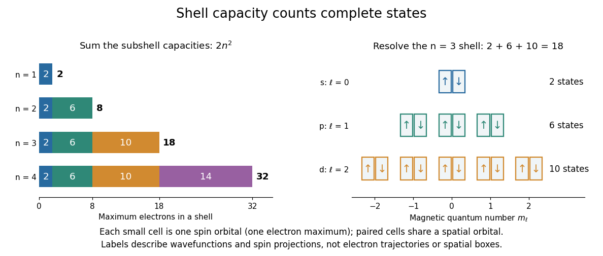
For example, $n=3$ allows $\ell =0,1,2$, conventionally $3s,3p,3d$. Their spatial orbital counts are $1,3,5$; their spin orbital counts are $2,6,10$. The sum is eighteen. The algebra behind “one per complete state” is short: two-particle antisymmetrization gives $u\wedge u=(u\otimes u-u\otimes u)/\sqrt{2}=0$, and the zero vector cannot be a normalized quantum state. Opposite-spin electrons in the same spatial orbital have distinct complete states, so their antisymmetric product survives.

This supplies a structural link to the periodic table: finite electron subshell capacities make repeated patterns of occupied electron configurations possible. It does not predict the exact ground state electron configuration or energy of a many-electron chemical atom. Different electron subshells overlap in energy, and electron interactions change their ordering. In particular, the periodic table period lengths are not simply successive $2n^2$ values: the third periodic table period has eight chemical elements, although the full $n=3$ electron shell has eighteen available states. A capacity counts available spin orbitals; an actual filling order requires a Quantum Hamiltonian.

In 1925, Wolfgang Pauli connected two puzzles: alkali metal doublets and their anomalous Zeeman effect, and the capacities of closed electron shells. His paper assigned the extra two-valued property to the optically active electron, rather than an angular momentum of the closed core. Its Paschen-Back effect classification used four quantum numbers; these historical labels should not be identified literally with modern $n,\ell ,m_{\ell },m_s$. The exclusion rule forbade matching all four. This connected resolved one-electron states with closed-group populations. An additional test was the missing triplet counterpart of the equivalent two-$s$-electron ground state in alkaline earth metals. Pauli explicitly claimed counts of allowed states, not their energies or ordering.^[ref]

The modern question is especially concrete: if a Quantum Hamiltonian has a lowest one-particle state, why cannot every electron occupy it? Minimizing energy answers which of the allowed quantum states is preferred; the Pauli exclusion principle determines which quantum states are allowed in the first place. Spectral lines then test energy differences between allowed multiparticle quantum states. A line count is not itself a direct count of occupied spin orbitals: transitions also depend on selection rules and the prepared quantum state populations. The observed anomalous Zeeman effect supplied constraints for the historical classification; the two-particle antisymmetrization below supplies the modern mathematical explanation of exclusion.

Equality of line integrals on two selected paths is a necessary test for a conservative vector field, but it is not sufficient. The paths may both miss the component responsible for nonzero curl.

For an explicit example, take $W(x,y,z)=(z-y,x-z,y-x{)}^T$. Its curl is the nonzero constant $2(1,1,1{)}^T$, so it is not a gradient field on ${\mathbb{R}}^3$. Nevertheless, on the plane $x=y$, the field equals $(z-x,x-z,0{)}^T$. Every tangent vector to that plane has equal first and second components, giving zero dot product with $W$. Thus every line integral of $W$ along a path confined to that plane is zero, regardless of endpoints or the path's shape.

In particular, a broken straight path and a genuinely curved path in that plane can have matching line integrals while revealing nothing about global path independence. To establish a conservative vector field, construct a vector-field potential, or verify the appropriate global criterion such as zero curl on a simply connected domain.