
Thermal penetration depth 2026-10-18
For the no-side-loss thermal diffusion wave, the thermal penetration depth is the distance over which the amplitude falls by and the wave phase lags by one radian. It is a periodic counterpart of the thermal diffusion length, with its numerical factor fixed by this definition. A shorter period probes a shallower region; a longer period increases sensitivity to the far-end boundary condition.
Combine the two massless neutrinos in into . In the parent rest frame, four-momentum conservation givesThe lower bound follows from the nonnegative Minkowski norm of the sum of two future-directed null four-vectors; the upper bound follows from . Substituting gives the displayed energy bounds. They are kinematic: they do not specify the weak interaction decay amplitude or the probability density function inside the interval.
If the charged daughter is also massless, put . A parent with Lorentz factor and speed in natural units producesHere is the daughter angle relative to the boost direction in the parent rest frame. Two opposite parent momenta therefore need not produce two opposite visible daughter momenta: the invisible system can recoil differently in each particle decay.
Positivity of a quadratic polynomial across a spectral gap Created 2026-10-18 Updated 2026-11-05
Let be a finite-dimensional Hermitian matrix and real. The spectral theorem gives in an orthonormal eigenbasis, soIf the spectrum avoids the closed interval, every factor product is positive. Consequently the quadratic form is positive for and zero for . More precisely it is bounded below by . This is a finite-dimensional instance of testing a spectral gap with a polynomial in the operator.
Solenoidal flux depends on the oriented boundary Created 2026-10-18 Updated 2026-10-25
Suppose two oriented surfaces have the same oriented boundary and bounds a volume inside a domain where the vector field is smooth and solenoidal. The divergence theorem gives zero flux through their closed union, proving the displayed equality. If a global vector potential exists on the relevant surfaces, the Stokes theorem proves the equality directly from their common boundary. The domain condition matters: a singularity inside the joining volume can obstruct the divergence argument.
Crystal X-ray spectrometer 2026-10-18
A crystal X-ray spectrometer selects a narrow wavelength interval by diffraction at known interplanar spacing and Bragg angle . For fixed diffraction order , a known lets an angular measurement determine . This reverses the crystallography problem of finding from a known wavelength.
Siegbahn's laboratory developed X-ray tubes and evacuated spectrographs for longer wavelengths. Rotating the crystal selected reflections; photographic plates recorded positions. Opposite-side exposures measured angles on both sides of the direct beam. Later tube instruments mounted a beam-defining slit opposite the plate holder. A separate double instrument compared two reflected beams with two ionization chambers. These were different instruments, not one universal assembly.[ref]
Manne Siegbahn, His Research by Hugo Atterling. Hugo Atterling, Manne Siegbahn: Development of precision spectroscopy; Work at Uppsala 1923–1927
The Nobel biography describes constant-temperature spectrographs and a precision angular scale read by diametrically opposed microscopes.[ref]
Manne Siegbahn - Biographical. Nobel Lectures, Physics 1922–1941; Biographical, paragraph beginning As a measure of the high precision; inspected collected volume pp. 90–91
Temperature control matters because thermal expansion changes ; an accurately read angle cannot compensate for an unknown interplanar spacing.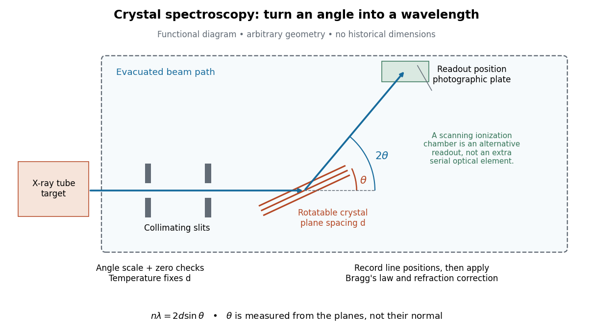

The schematic separates preparation, selection and readout. An X-ray tube target supplies Characteristic X-rays with a possible bremsstrahlung background. A collimator limits incident directions; evacuation reduces air X-ray attenuation. Rotating the crystal brings different wavelengths into reflection. A photographic plate stores line positions over an exposure, whereas an ionization chamber can measure collected electric charge at successive angles. Neither readout alone establishes absolute wavelength: an angular zero, angular-scale calibration, diffraction order, and any required refraction correction enter the inference. Narrower slits reduce accepted angular spread but also reduce signal; a weak line can become harder to locate despite a narrower instrumental response.
A control reported in Siegbahn's lecture photographed a line system with copper-sulphate and calcium-sulphate crystals. Irregular relative shifts around copper's characteristic frequency supported anomalous dispersion; the arrangement excluded differing absorption across that frequency as the explanation.[ref]
The X-ray Spectra and the Structure of the Atoms by Karl Manne Georg Siegbahn. Nobel Lectures, Physics 1922–1941; Printed pp. 88–89, final experiment
A finer angular scale alone cannot remove this physical refraction correction. Verifying a satisfying assignment Created 2026-10-18 Updated 2026-10-25
For a CNF input with Boolean variables, Boolean clauses, and Boolean literal occurrences, first check that the supplied Boolean valuation gives each input Boolean variable exactly one truth value. Evaluate each Boolean literal by lookup or logical negation, each Boolean clause by logical disjunction, and the Boolean formula by logical conjunction. Indexed Boolean variables and constant-cost lookups give an operation count; with a finite binary string encoding the check still takes polynomial time. Thus a satisfying assignment is a certificate in computational complexity for SAT, proving that SAT belongs to NP. Finding it by exhaustive checking can require candidate Boolean valuations; this enumeration cost is not a lower bound on every possible SAT algorithm.[ref]
CS 252, Lecture 8: Constraint Satisfaction Problems (Carnegie Mellon University). CS 252, Lecture 8: Constraint Satisfaction Problems, p. 3, §3 opening paragraph: assignments as certificates and membership in NP
A single optical shift represents pressure only to the extent that the calibration's mechanical and thermal conditions apply. Under hydrostatic stress, all directions have the same compressive normal stress. Under deviatoric stress, differently oriented ruby grains can respond differently; spatially varying pressure can also superpose shifted lines. These mechanisms can produce different optical signals at equal mean pressure.[ref]
Stress Measurements in Alumina by Optical Fluorescence: Revisited by Robert F. Cook and Chris A. Michaels. Sections 1–2: stress-sensitive fluorescence shifts and crystallographic stress components
The 2001 account describes scanning local line positions and measuring line width over an extended region. The former resolves spatial differences; the latter supplies a rapid warning.[ref]
High Pressure X-Ray Crystallography With the Diamond Cell at NIST⁄NBS by Gasper J. Piermarini. Section 4.2, Methods I and II
Neither a broadened line nor a narrow one uniquely determines the stress tensor. Instrument resolution, temperature variation and unresolved overlapping signals can also affect width. A small observed region can have a narrow line while differing from another region. Compare locations, reference traces and instrument settings before treating width as evidence for a particular mechanical explanation. These are proposed diagnostic checks, not additional historical controls attributed to the 1975 experiment.
Temperature is another independent input. A useful local expansion is : one measured shift cannot determine both unknowns. Measure or control temperature, or supply a second independently calibrated observable. The coefficients need not remain constant across a large range. Even when a pressure sensitivity transfers over some temperatures, the reference line, line width and practical readout quality can change.
The historical high-temperature account reports degrading pressure measurement quality above about .[ref]
High Pressure X-Ray Crystallography With the Diamond Cell at NIST⁄NBS by Gasper J. Piermarini. Section 4.1, high-temperature cell and readout-quality discussion
Ruby pressure uncertainty worked example 2026-10-18
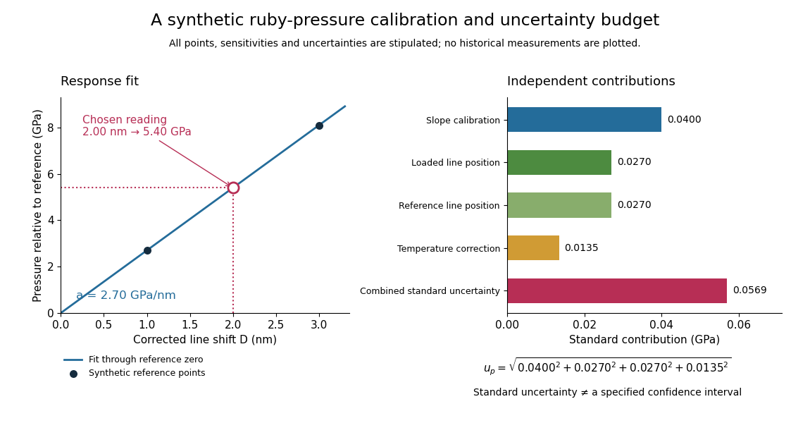
Construct a synthetic local calibration to show the calculation independently of the historical data. Choose reference pairs , with shifts in and pressures in . The reference zero is already subtracted. Treat the shifts as exact for this fit and give the three reference pressures equal weights. Minimizing the ordinary least squares objectiveand setting its derivative to zero givesThe regression residuals are . Their weighted moment vanishes, as required by the least-squares normal equations. An unknown reference offset requires fitting an intercept instead; forcing it to zero can bias the slope. If shift errors matter, this elementary fit is insufficient.
Synthetic ruby pressure scale: fitting the response and propagating measurement uncertainty
. Original stipulated reference points and calculations, not measured historical calibration. The left panel shows the fitted slope and a chosen reading. The right panel separates independent contributions to standard uncertainty; bar lengths are standard contributions, which combine by sums of squares. The assigned slope standard uncertainty includes a hypothetical reference-scale contribution and is not estimated from the three residuals. Details.
Use the local measurement modelHere denotes pressure relative to the reference, is calibrated sensitivity, and is a local wavelength sensitivity to temperature at fixed pressure. Choose , and a reading at . The inferred pressure is . These coefficients and readings are stipulated, not measured ruby constants. With the same pressure, a increase in temperature would add to the shift in this model; neglecting it would overestimate pressure by .
Assign independent standard uncertainties , and for the temperature difference. Here is an independently assigned calibration uncertainty, not an estimate from the regression residuals above; treat as exact in this example. First-order propagation of uncertainty follows by differentiating the measurement model:The four standard contributions are , giving . This is a standard uncertainty, not automatically a interval. Correlated reference and loaded wavelength readings require the corresponding covariance term; common wavelength-axis drift may cancel in their difference. Uncertain , nonzero , model inadequacy and unresolved deviatoric stress require a broader budget. Taking more optical readings reduces some random errors while leaving a common reference-scale error.
Ruby calibration against sodium chloride 2026-10-18
The 1975 experiment mixed powdered sodium chloride and 0.5%-chromium ruby in a 4:1 volume ratio. An Inconel gasket, initially thick with a hole, held the powder and 4:1 methanol–ethanol. At , X-ray diffraction rings on film away gave salt compression; a reference equation of state assigned pressure. After decreasing load, they waited at least five hours and bracketed diffraction exposures with readings to check drift.[ref]
Calibration of the pressure dependence of the R1 ruby fluorescence line to 195 kbar by Gasper J. Piermarini and others. pp. 2774–2775, Experimental Procedures
The recommended linear slope was , with a fit confidence interval of , to . Reference-scale systematic measurement uncertainty remained separate. Above about the medium was only quasihydrostatic; separate range fits checked consistency.[ref]
Calibration of the pressure dependence of the R1 ruby fluorescence line to 195 kbar by Gasper J. Piermarini and others. pp. 2775–2776, Table I and recommended calibration; p. 2778, pressure-distribution discussion
The logical chain is compression to reference pressure, paired with optical shift, then a fitted response. X-ray diffraction supplies the reference comparison during calibration; subsequent ruby readings transfer that scale to other samples. The reference equation of state is therefore part of the meaning of the reported pressure. Changing it can move all calibrated readings together, even if the optical measurements repeat perfectly. A regression residual tests agreement with the chosen reference within the sampled conditions; it cannot independently certify that reference.
Ruby R-line shift 2026-10-18
The ruby R-line shift compares the same emission feature under two conditions. It is distinct from the Stokes shift, which compares absorption and emission features. In ruby, chromium ions in the corundum crystal provide the electronic transitions; compression changes their local environment and transition energies.[ref]
Stress Measurements in Alumina by Optical Fluorescence: Revisited by Robert F. Cook and Chris A. Michaels. Introduction and hydrostatic-pressure discussion: chromium fluorescence in alumina and stress-sensitive R lines
For consistently defined vacuum wavelengths, the reciprocal relation givesThus a positive wavelength shift means a negative reciprocal shift, and gives lower photon energy; is the Planck constant and the speed of light. For spectroscopic wavenumber, use vacuum wavelength and keep that convention consistent. A calibration specified in air wavelength must retain its convention or be converted consistently. The reciprocal relation is nonlinear: a line exactly linear in is not exactly linear in .
For a purely mathematical check with chosen vacuum wavelengths and , the reciprocal shift is . The small-shift approximation gives , about too large in magnitude. These chosen values illustrate the conversion; they are not measured ruby lines or an additional pressure calibration.
In 1938, Isidor Isaac Rabi, Jerrold Zacharias, Sidney Millman and Polykarp Kusch introduced molecular-beam magnetic resonance. Their 1939 account describes a heated oven, vacuum slits, inhomogeneous A/B magnetic fields with opposite gradients, and a uniform static C magnetic field. Conductors supplied transverse oscillatory radiofrequency (RF) fields. Transitions spoiled refocusing, reducing the tungsten-filament detector signal. Alignment compared A-only and B-only attenuation; C-field sweeps at fixed RF frequency limited oscillator pickup. Matching frequency/field ratios across compounds checked nuclear assignments. Magnetic field calibration limited absolute magnetic moments; weak intervening fields caused unwanted transitions.[ref]
The Molecular Beam Resonance Method for Measuring Nuclear Magnetic Moments by Isidor Isaac Rabi and others. Rabi, Millman, Kusch and Zacharias, Physical Review 55 (1939), pp. 526–533; Figs. 1–5; Apparatus, Procedure and Results; p. 526 references to the 1938 reports
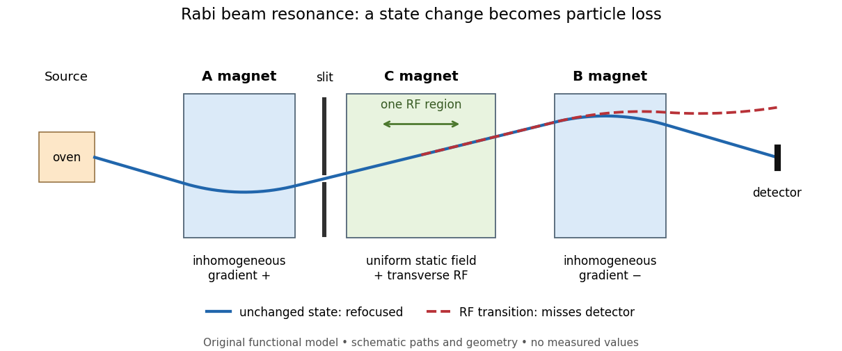
Functional beam selector: unchanged states refocus; RF transitions cause detector loss
. Original functional diagram of the Rabi molecular beam magnetic resonance experiment; paths are schematic and not to scale. Details.
The readout has a useful logical structure: A and the apertures admit trajectories correlated with a magnetic moment projection; B tests whether that projection has survived C. The two deflectors compensate for unchanged states, whereas a changed projection experiences a different force in B. A dip followed by recovery as the static magnetic field passes through resonance is therefore a population-sensitive signal. A comparison with RF absent or far from resonance is the natural baseline in this functional model; RF pickup, drift or background loss must not be mistaken for a state transition. A dip alone does not establish a pure initial quantum state or resolve an entire time-domain Rabi cycle.
This beam method measures transmitted particles after state-dependent deflection. The later bulk nuclear magnetic resonance methods of Felix Bloch and Edward Mills Purcell instead use a macroscopic sample and detect nuclear induction or RF absorption; NMR spectroscopy builds on that bulk setting. The common resonant coupling does not make their preparations or readouts interchangeable.[ref]
Our History by Stanford University Physics Department. Physics Department, Our History, The Middle 1930s through the 1960s, paragraphs on nuclear induction in condensed matter and spectroscopy
[ref]Harvard’s Nobel Laureates in Physics by Harvard University. Harvard’s Nobel Laureates in Physics, Edward M. Purcell section, nuclear magnetic resonance absorption
Driven two-level Rabi model 2026-10-18
Choose an isolated pair of energy levels, with ground state and excited state . Use the Pauli matrices in the ordered basis , so . After subtracting the mean energy, prescribe the laboratory Hamiltonian operatorThe unperturbed energy gap is , the drive has angular frequency , and fixes its oscillation phase at the chosen time origin. All of , , the Rabi angular frequency and the Rabi detuning are in radians per second; ordinary frequency is angular frequency divided by . In particular, here is the coefficient multiplying the cosine in , not twice that coefficient.
Write with . Transforming the Schrödinger equation gives . The rotating-wave approximation drops terms at angular frequency , leavingThis approximation requires , and an interaction duration over which omitted corrections remain small. It also assumes that other energy levels can be neglected. Resonance alone does not justify either assumption. An exactly co-rotating drive has no discarded counter-rotating component; the linearly oscillating laboratory drive above does.
The Pauli matrix multiplication law gives . Separating even and odd terms of the matrix exponential therefore proveswith the continuous limit when . Starting from , the upper probability amplitude is . The Born rule givesThe rotating transformation only changes the quantum phases of these basis states, so their laboratory populations are the same. Rabi detuning tilts the rotation axis of the Bloch vector: it increases the oscillation rate to but caps the transferred population at . A fixed drive oscillation phase cancels from this single-pulse population when the initial state is . It still fixes the relative quantum phase of a resulting quantum superposition and matters when another pulse supplies a phase reference.
Resonance envelope of a Rabi transition Created 2026-10-18 Updated 2026-10-20
In the Driven two-level Rabi model, the transition probability is . Maximizing over time at each detuning gives a Lorentzian line shape, with first maximizing time and full width at half maximum in angular frequency. The amplitude parameter must use the specified Rabi angular frequency convention.
Double-pass quarter-wave plate 2026-10-18
For a reciprocal ideal quarter-wave plate followed by a mirror at normal incidence, use the same fixed transverse laboratory axes for the forward and returning Jones vectors. If the axes coincide with the plate's fast and slow axes, each pass has Jones matrix up to a common phase factor. A polarization-independent mirror has scalar reflection coefficient , so the returned Jones vector is . The plate acts twice as a half-wave plate, rather than undoing its phase retardation.
For input linear polarization at angle to the fast axis, the returned line is at modulo . At it is perpendicular to the original line. An axis-aligned input instead returns along the same line. General elliptical polarization requires its full input Jones vector; no unique returned state follows from the word “polarized” alone. The propagation direction reverses, so comparing descriptions of circular polarization must also specify the viewing convention.
Pure-polarization preparation with two quarter-wave plates Created 2026-10-18 Updated 2026-10-20
Two rotatable ideal quarter-wave plates can transform a fixed circular polarization into any pure polarization represented by a Jones vector. Use time dependence , and input . Every target polarization ellipse can be written, up to a common phase, as , with signed ellipticity angle . The first quarter-wave plate at produces linear polarization at . The second, at , therefore produces the required target. The two angles supply the two independent parameters of pure polarization.
Fractional quantum Hall effect Created 2026-10-18 Updated 2026-10-20
The fractional quantum Hall effect is quantized transverse sheet conductivity at fractional filling factors, produced by interacting electrons. The Laughlin wavefunction describes the sequence , with odd , including .[ref]
For an original ideal readout example, take a Hall bar on the plateau with negligible longitudinal sheet conductivity. The quantum Hall conductivity tensor inversion givesHere is the von Klitzing constant; denotes transverse electrical resistance, rather than the bulk Hall coefficient. Thus a fractional sheet conductivity corresponds to a larger transverse electrical resistance. The fraction labels a collective quantum state: it does not mean that each electron has acquired one third of its usual electric charge.
Integer quantum Hall effect Created 2026-10-18 Updated 2026-10-20
On an ideal integer plateau, the magnitude of transverse sheet conductivity is , where is a positive integer, while the longitudinal sheet conductivity vanishes. The measured transverse electrical resistance is then . Both statements matter: inverting a conductivity tensor mixes its longitudinal and transverse components, as the quantum Hall conductivity tensor inversion shows.
Hulse-Taylor timing experiment 2026-10-18
The surprise was a pulsar whose apparent period would not stay fixed. Russell Alan Hulse's Arecibo search used a multichannel receiver, pulsar dedispersion and computer searches over period and pulse width. Follow-up at higher time resolution retained the changing period, excluding inadequate sampling as its explanation. The observed variation exceeded the expected terrestrial Doppler shift; a predicted reversal from decreasing to increasing period appeared on 16 September 1974.[ref]
The Discovery of the Binary Pulsar by Russell Alan Hulse. The Discovery of the Binary Pulsar, lecture delivered 8 December 1993, pp. 53–58 and 62–65, Figures 3–4 and 8–10
The 1975 analysis fitted an eccentric Kepler orbit to Doppler shifts inferred from about 200 five-minute period measurements over ten days. That discovery fit was not yet the later precision arrival-time experiment.[ref]
Discovery of a Pulsar in a Binary System by Russell Alan Hulse and Joseph Hooton Taylor Jr.. L51–L52, section II, Tables 1–2, Figure 1 and equations 1–4
An orbit explains both signs of the apparent period change without requiring the stellar rotation to alternate between speeding up and slowing down. There are unlisted articles, also show them or only show them.