
Residual resistivity Created 2026-10-18 Updated 2026-11-05
The residual resistivity is the low-temperature electrical resistivity remaining in a normal metal when thermally excited scattering becomes negligible. Static disorder, impurities and boundaries can relax carrier momentum without requiring a thermal population of phonons. Its value depends on sample purity and structure; a superconducting transition is a different phenomenon.
Resistivity tensor Created 2026-10-18 Updated 2026-11-05
The resistivity tensor is the matrix relating electric field to current density in linear local transport. It is the matrix inverse of the conductivity tensor, not the componentwise reciprocal. A Hall response produces antisymmetric off-diagonal components. In a multicarrier system, the conductivities add because each species sees the same electric field; invert only after summing the species' conductivity tensors.
Rabi pi pulse 2026-10-18
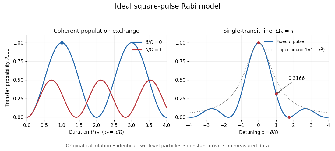
For a constant-amplitude square pulse on resonance, a Rabi pi pulse lasts and gives in the rotating frame. A half-duration pulse prepares . The quantum pulse area determines these rotations only under the stated resonant, constant-axis assumptions; a detuned drive rotates about a different axis.
As an original numerical illustration, choose and hence . These are chosen model parameters, not historical apparatus settings. Holding that duration fixed givesThus , , and . The last zero comes from completing a full rotation about the tilted axis, rather than switching the drive off. At zero Rabi detuning, doubling the pulse duration restores the ground-state population; continuous driving does not keep transferring population irreversibly.

Rabi detuning Created 2026-10-18 Updated 2026-11-05
The Rabi detuning is the unperturbed transition angular frequency minus the drive angular frequency in this convention. Its sign controls the longitudinal rotation of the Bloch vector; the single-pulse population formula is even in . Reversing the definition of Rabi detuning requires reversing its sign in the rotating-frame Hamiltonian operator as well.
Rabi angular frequency Created 2026-10-18 Updated 2026-10-20
The Rabi angular frequency is the on-resonance population oscillation rate in the specified Driven two-level Rabi model. The rotating-frame off-diagonal Hamiltonian operator entry has magnitude . Stating this convention avoids a factor-of-two ambiguity between drive coefficients and oscillation rates. The generalized rate off resonance is .
Two-current resistor model 2026-10-18
Consider two identical magnetic layers separated by a nonmagnetic layer, between reservoirs that impose the same terminal electric potential difference on both spin channels. Neglect spin-flip scattering and assume each layer obeys Ohm's law. In a magnetic layer, define positive channel electrical resistances . Let the spacer contribute to each channel. These are circuit parameters, not measured iron or chromium resistivities.
For parallel layer magnetizations, one channel meets and the other . For opposite layer magnetizations, each meets one , one , and the spacer. The two channels share the same terminal electric potential difference and run in parallel. Writing givesThe inequality is algebra, given the specified network. It shows how a difference between spin-channel responses can yield a difference between magnetic configurations even though all the constituent resistors are ohmic.
For chosen , , , the parallel channels have total electrical resistances and , while the opposite-alignment channels each have . Thus and . At a common terminal electric potential difference , the total electric currents are and , respectively.
Gaussian spectral doublet resolution 2026-10-18
A spectral doublet comprises two neighbouring spectral lines. Resolving it requires information about the line response, relative strengths and noise, not only precision in reading an angle. Choose two equal angular responses shaped as Gaussian functions with common standard deviation and separation . If is angular displacement from their midpoint, their summed signal isThese are assumed response shapes, not a measured Siegbahn frequency spectrum. By symmetry , andThe midpoint changes from a maximum to a minimum at . For this particular equal-width, equal-height model, two distinct maxima occur when . Each isolated Gaussian function has full width at half maximum ; the two-maxima threshold is therefore about times that width.
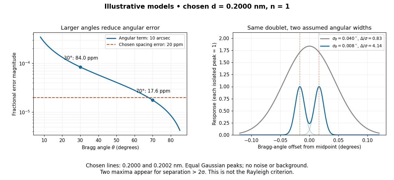

In this chosen model, the two Bragg angles are and . Their separation is times for , giving one maximum, and times for , giving two. Sharpening the response can reveal the doublet without changing either emitted wavelength.
The Rayleigh criterion uses a first-zero convention for specified diffraction patterns. A Gaussian function has no finite zero, so its two-maxima threshold is not the Rayleigh criterion. Neither convention is a universal inference limit: known response shapes and adequate signal-to-noise ratio can support estimating a separation before two visible maxima appear. Unequal strengths, background, finite sampling and uncertainty in the response can make that inference much harder. Measurement resolution, the precision of an isolated line's centre and absolute wavelength accuracy should therefore be reported separately.
Relative X-ray wavelength calibration 2026-10-18
For two lines measured with the same interplanar spacing at the same temperature, division of Bragg's law givesThe common cancels. Consequently a precise wavelength ratio can coexist with an uncertain conversion to SI length. In contrast, angular calibration errors generally survive: a shared small zero offset changes the inferred ratio fractionally by approximately . Nearby lines partially cancel this effect, but widely separated angles need not. Different crystals, temperatures or refraction corrections also prevent unqualified cancellation.
Bragg wavelength error propagation 2026-10-18
Differentiate Bragg's law at fixed correctly assigned diffraction order:Divide the second equality by the first. For small signed changes,The Bragg angle error must be in radians. An error quoted for detector deflection must first be halved. The expression is a first-order Taylor expansion; an unknown diffraction order is a discrete assignment error, not an infinitesimal perturbation.
For error bounds, add magnitudes. For independent zero-mean random errors with standard deviations , variance addition instead givesCorrelated errors require a covariance term. A shared calibration bias does not become independent merely because many line positions are measured.
With a chosen angular error arcseconds, , the angular contribution is at and at . Larger Bragg angles reduce this contribution because decreases. For a nearby spectral doublet, the inverse relation is : a fixed fractional separation spreads farther apart angularly at large Bragg angle.
This does not permit unlimited improvement. The geometry requires ; a desired wavelength might not have an accessible large-angle reflection with the chosen crystal. Higher diffraction orders can reach larger Bragg angles but their strengths depend on the crystal lattice structure factor. Finite crystal response, slit widths and source size remain relevant. An error in , including uncorrected thermal expansion, remains even when the angular term is small. Very near , the leading angular derivative vanishes and the second-order Taylor expansion matters.
For a lossless nonmagnetic uniaxial optical medium, the electric displacement field of a plane electromagnetic wave is perpendicular to its wavevector. The magnetic field is perpendicular to the plane containing the electric field and wavevector, while the Poynting vector is perpendicular to the electric field in that same plane. Thus the angle between and equals the walk-off angle between energy flow and phase propagation. At normal incidence on a parallel slab of thickness , a lateral separation of the ordinary and extraordinary exiting rays gives , while . The output rays can be parallel even though their internal energy paths differ.
Complex analytic representation of biharmonic functions Created 2026-10-18 Updated 2026-10-20
If are holomorphic functions, both real and imaginary parts of solve the biharmonic equation. In Wirtinger derivatives, , so is harmonic and its next Laplacian is zero. This construction gives local representations of planar solutions of the biharmonic equation; it is useful for the biharmonic stream function for planar Stokes flow.
Lorenz number 2026-10-18
The Lorenz number is the ratio . The Sommerfeld value applies under the assumptions of the Wiedemann-Franz law. The ratio must use electronic thermal conductivity if lattice heat flow is appreciable.
Thermal and electrical relaxation times in metals Created 2026-10-18 Updated 2026-11-05
For a degenerate isotropic parabolic electron band, electrical conductivity is and electronic thermal conductivity is . Their ratio is , where is the Lorenz number. Nearly elastic scattering that relaxes charge and heat currents similarly gives and the Wiedemann-Franz law. Inelastic scattering can relax heat current and directed momentum differently, invalidating the simplest identification even in a good metal.
Worked two-length tensile compliance example 2026-10-18
The following values are stipulated arithmetic inputs, not measurements of a material. Take and lengths , . At forces , stipulate crosshead displacementsThe two different initial offsets deliberately test the use of intercepts. Linear regression of gives , andTheir reciprocal spring constants are and . The compliance-versus-length slope isso the recovered Young's modulus and machine compliance areThe corresponding apparatus spring constant is .
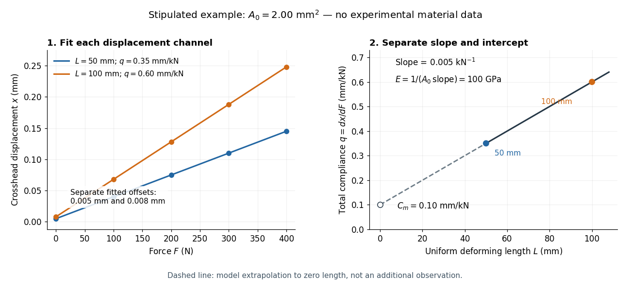
Stipulated displacement fits separate length-dependent compliance from apparatus compliance
. Original calculated example, not experimental material data. Left: independent linear displacement fits at lengths 50 and 100 millimetres retain their different offsets. Right: the line through the two compliance values has slope 1/(EA0) and intercept Cm. The dashed segment extrapolates the model to zero length; it is not a third observation. Details.
Check the reconstruction at . The machine contribution is , and the two specimen contributions are and . Adding the respective offsets gives the stipulated and . An extensometer spanning on either ideal uniform specimen would instead read extension: engineering strain , at engineering stress . Their ratio is again . Ignoring machine compliance gives apparent moduli and even after removing the offsets. No yield point or real material identity is implied by these stipulated linear inputs.
Angular response of a gravitational-wave separation Created 2026-10-18 Updated 2026-10-25
For a short pair of stationary test particles in transverse-traceless gauge, spatial coordinates stay fixed while the measured proper length changes. In background signature , let and . A coordinate separation of length at angle hasThe plus polarization and cross polarization differ by a -degree rotation of their principal axes. With background signature and the same numerical spatial perturbation, the sign reverses because the positive spatial metric is then rather than . Consistently redefining the signed strain leaves the physical effect unchanged.
Total divergences in a variational principle Created 2026-10-18 Updated 2026-11-05
Adding to a mechanical Lagrangian changes its action by . Fixed endpoint variations therefore leave its bulk Euler-Lagrange equations unchanged. For fields, adding changes the action by a boundary flux. The same conclusion holds for compactly supported variations or appropriate fixed boundary data. If depends on field derivatives, those boundary data must also control their variations. Such terms can still change canonical momenta, boundary observables, and representatives of Noether currents; equivalence of bulk equations does not mean that every boundary-value problem is identical.
Suppose a constant Hamiltonian operator has a complete discrete orthonormal basis of energy eigenstates, . Expanding an initial pure state and applying the time-evolution operator term by term givesA projective measurement resolving these basis vectors therefore assigns the same Born rule probability to each label at every time. An energy measurement groups labels sharing the same energy eigenvalue: is also constant. If , their probability amplitude ratio instead evolves asOnly energy differences enter this relative quantum phase. Adding a constant to the Hamiltonian operator multiplies the entire pure state by , a global phase, and leaves the density operator unchanged.
For a fixed observable , the expectation value can nevertheless vary:Terms joining distinct energy eigenvalues can oscillate; diagonal terms cannot. If , these terms between different energies vanish, so the expectation value is constant. This distinguishes conservation of energy from the stronger claim that every observable is stationary.
An energy eigenstate has only a global phase evolution and is a stationary state. A quantum superposition entirely within one degenerate energy eigenspace is also an energy eigenstate and is stationary. For a general density operator in finite dimension, stationarity under a constant Hamiltonian operator means : differentiating proves necessity, and commuting through the exponential proves sufficiency. Merely fixing the diagonal energy populations does not fix the off-diagonal quantum coherence.
Floquet operator 2026-10-18
For a periodic Hamiltonian , the Floquet operator is the unitary operator evolving a quantum state through one complete period, at a fixed starting phase of the drive. The composition law gives . Choosing a different starting phase conjugates by a unitary operator, so its eigenvalues are unchanged.
Quantum propagator 2026-10-18
The position-space kernel of the time-evolution operator propagates a wave function by . It tends to as . A retarded convention multiplies it by the Heaviside step function: . This convention obeys ; dividing by gives the Green function with a unit delta source. The time phase for an energy eigenstate is always .
Thomas-Fermi screening length 2026-10-18
The Thomas-Fermi screening length is the exponential decay scale of a statically screened potential in the local degenerate-electron approximation. For a three-dimensional parabolic free electron model, , so . At fixed mass and background permittivity it scales as , rather than the classical Debye density power at fixed temperature.
There are unlisted articles, also show them or only show them.