The Reynolds number compares inertial and viscous effects:where is fluid mass density, a characteristic swimming speed, a characteristic body length, and the dynamic viscosity. Both swimmers are in the same fluid, so the fluid properties cancel from the ratio:For an order-of-magnitude estimate, take , , and . With water values and , these giveand henceThe dimensions and swimming speeds are estimates, so this ratio is not a universal species-independent constant. Its physical significance is robust: viscous forces dominate the bacterium's motion, whereas fluid inertia is crucial for the whale.
There is a source error to resolve first. For a drag coefficient defined by , the velocity relaxation time is . The mass and drag coefficient in the PDF's exponential are interchanged: is dimensionless, whereas is not. The consistent mean relaxation law is therefore .
A mean relaxation law alone does not determine a variance. Use the usual thermal Langevin equation, with a bath at temperature and the fluctuation-dissipation relation for a Langevin particle:Here the calculation is for one component in Cartesian coordinates. With fixed initial position and velocity, integration gives the mean displacementIntegrating the stochastic part of the velocity once more gives the centered displacementThe delta correlation reduces its variance to a single integral:This is the integrated Ornstein-Uhlenbeck displacement for a prescribed initial velocity. Its short-time variance is ; at long times it is . Thus the diffusion coefficient isIf the requested mean-squared fluctuation instead refers to the conventional equilibrium mean squared displacement, the initial velocity is also averaged over its thermal distribution, with and . Its contribution adds , givingThis has the ballistic limit and the same diffusive limit . For fixed nonzero , the uncentered mean square instead equals the first boxed variance plus . In three independent spatial dimensions, the centered variances add, and the long-time result is . Stating the initial-velocity convention is necessary to distinguish these finite-time formulas.
Two examples are sodium dodecyl sulfate, with a negatively charged sulfate head and a hydrocarbon tail, and cetrimonium bromide, with a positively charged ammonium head and a hydrocarbon tail. Both are amphiphiles: one region is hydrophilic and another is hydrophobic.
In water, the hydrophobic effect favors association of the tails into a core, reducing their exposed area while the hydrated heads remain outside. This can lower the total Gibbs free energy despite loss of translational entropy. Head-group repulsion, interfacial cost and chain-packing constraints oppose unlimited growth, so finite micelles are favored under suitable conditions above the critical micelle concentration.
The appropriate geometric measure is the amphiphile packing parameter:For a spherical micelle with tails and core radius , the volume and area relations are and . Dividing gives , so a sphere fits without overextending a tail if . Here andThus the packing model predicts spherical micelles. This is a preferred aggregate geometry, not a claim that concentration, temperature or ionic conditions can never alter the morphology.
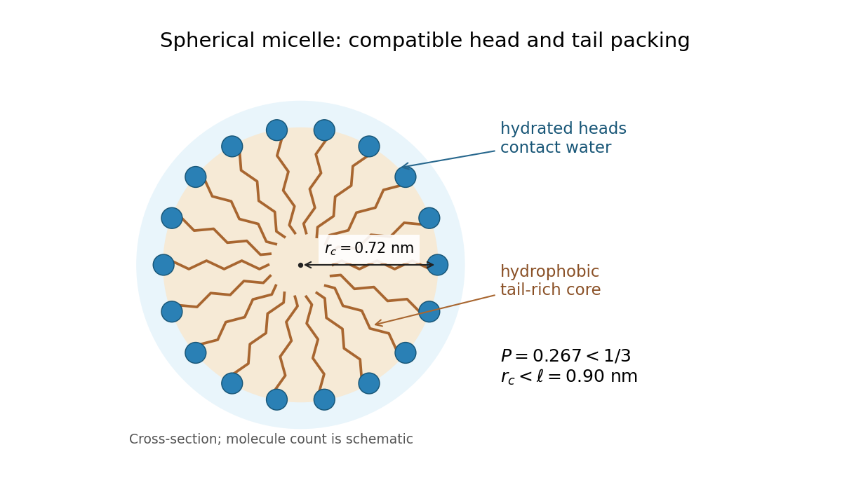
An original cross-section of spherical micelle packing
. Hydrophilic heads face the water and hydrophobic tails fill the core; the drawing illustrates packing geometry rather than a measured aggregation number. Details.
Diffusion and mobility. For a dilute isolated sphere in a Newtonian fluid, Stokes's law gives the drag magnitude , where is the dynamic viscosity and is the hydrodynamic radius. The mechanical mobility is therefore ; the translational hydrodynamic mobility matrix is .
To relate mobility to diffusion, put the particles in a weak external potential energy . Their drift speed is . For number density , the sum of drift and Fick's first law fluxes isAt thermal equilibrium, the Boltzmann distribution gives , and the net flux is zero. Substituting into yields . Thus the Stokes–Einstein relation isHere is the Boltzmann constant and is absolute temperature. The assumptions include a no-slip approximately spherical particle, a continuum fluid, a small particle Reynolds number, and negligible hydrodynamic interactions with other particles or boundaries.
Gravitational sedimentation. The buoyant force must be included, since the mass of displaced water is comparable to the protein mass. Using givesso the buoyant mass in the stated spherical model isThe drag coefficient is . At terminal speed, , soIgnoring buoyancy would give and would not use the supplied water density. This calculation treats the stated radius as both the hydrodynamic radius and the radius determining displaced volume; a real hydrated protein can require a separately measured partial specific volume.
Electrical drift. In the specified simple electrophoresis model, terminal force balance is . Thereforewhere is the electrophoretic mobility and the elementary electric charge. For the given positive beta-lactoglobulin charge,in the direction of the electric field. This exceeds the gravitational sedimentation speed by about .
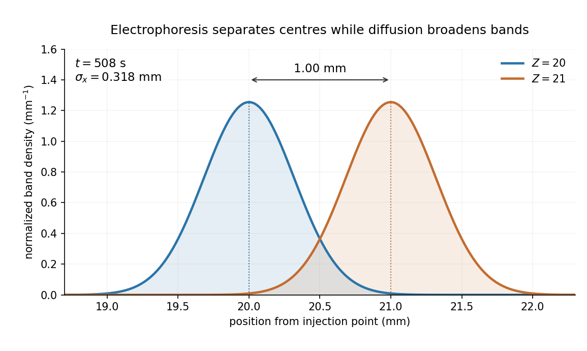
Separation time. The two populations have equal drag coefficients because their radii are equal. Their difference in drift speed is therefore set by one elementary charge:Starting with coincident band centres, their separation is . HenceAt that time the original band has travelled and the mutant . Their masses do not enter this ideal electrical force balance: equal-radius particles with different masses but the same charge would have equal electrophoretic mobility in this model.
Practical discrimination. A one-charge difference is enough for the stipulated separation, so the method is sensitive to mutations that change effective charge or friction. It cannot distinguish every mutation: substitutions that preserve charge and hydrodynamic size need not separate. Buffer pH changes protein ionization, and realistic electrophoresis also involves the ionic atmosphere, electro-osmosis, walls or gel interactions, and finite band widths.
For example, the Stokes–Einstein relation at gives . For an initially narrow band, diffusive broadening of electrophoretic bands givesat the calculated separation time. Thus the centres are about diffusion standard deviations apart, rather than forming infinitely sharp bands. The stated centre-separation criterion is achievable in the model, but actual resolution also depends on the loading width and other dispersion mechanisms.

Equivalent centrifugal acceleration. For the original protein to attain its electrical drift speed by sedimentation, its buoyant centrifugal force must equal :ConsequentlyThis is the acceleration at the protein's position in the rotating solution; no rotation rate can be assigned without a centrifuge radius. If the intended comparison is instead the relative separation speed of the two bands, use , since their displaced volumes are equal. Matching then gives . In that separation experiment the heavier original protein moves faster centrifugally, whereas the more highly charged mutant moves faster electrically.
Solvent quality. The Flory interaction parameter measures the free-energy cost of polymer–solvent contacts relative to like contacts. In the simplest lattice model,where is the coordination number and the values are contact energies. For lattice-site volume , the effective two-segment excluded volume is . Its sign determines the leading tendency of a long dilute flexible chain.
For , : a good solvent favors a swollen coil because segment encounters are effectively repulsive. For , the leading attraction and repulsion cancel, giving approximately ideal chain statistics. For , effective attraction favors contraction in a poor solvent, eventually producing a compact polymer globule under sufficiently poor conditions. This does not mean that every finite-chain solution with is automatically phase-separated; that also depends on composition and chain length.
The condition is the theta temperature condition for that polymer–solvent pair. For an energetic model , it occurs at . More generally, if , it occurs when . It is not the absence of all intermolecular interactions and does not require the polymer and solvent to be chemically identical.
Chain dimensions. Interpret as the root-mean-square end-to-end distance of a polymer chain. Let denote the supplied statistical step length, calibrated to the same count as the degree of polymerization. At the theta condition, random-walk statistics giveFor a good solvent, the Flory approximation balances entropic stretching and two-segment interaction:Minimization gives , henceThus the familiar good-solvent scaling is when its nonuniversal solvent-quality amplitude is suppressed. With the additional lattice estimate , the more explicit form is . This swollen-coil estimate is used away from the narrow theta crossover; it must not be extrapolated to predict as . The crossover occurs when is of order one. Nearer theta, the ideal-coil size supplies the appropriate limit.
Numerical sizes. The theta value isFor , the plain good-solvent scaling givesIf the solvent-quality amplitude is retained with , it instead givesThe distinction is an explicitly stated modeling convention: the question does not give a microscopic site volume or an absolute swollen-coil prefactor. Both estimates describe a coil larger than the theta coil. Here , so a swollen-coil estimate is reasonable. Neither result is an exact microscopic prediction from the supplied data alone.
Overlap concentration. The polymer overlap concentration corresponds to one chain per coil volume. Using the scaling convention givesThe first is chain number density; the second counts repeat units. Thus the repeat-unit molar concentration is approximately . If the lattice-site volume is taken as , this is equivalentlyFor a mass-concentration estimate, a polystyrene repeat unit has molar mass about , so this scaling convention givesThere is no sharp coil surface fixing an exact numerical prefactor. For example, using the often adopted geometric definition , with the ideal chain radius of gyration , gives . The invariant content is one chain per coil volume and the theta scaling ; the radius and coil-volume convention must accompany a numerical value.
Osmotic pressure. In the given lattice expression, is a dimensionless polymer volume fraction, not a dimensional number density, and is the mixing free energy per lattice site. Introduce to obtain a physical osmotic pressure. If is the number of sites and , differentiation of with respect to the solvent count at fixed chain count givesBalancing this change in solvent chemical potential against the pressure contribution gives . For composition-independent ,and therefore the osmotic pressure in Flory-Huggins solution theory isExpanding the logarithm as givesThe first term is with now denoting chain number density: a whole chain supplies one translational contribution. The sign of the quadratic correction reproduces the solvent-quality classification. It is positive for a good solvent, zero at the theta temperature, and negative for a poor solvent. This is the same two-segment interaction that swells or contracts a single coil. At theta, a positive third-order contribution remains; the chain is approximately ideal in its large-scale conformation, not a gas of segments with no interactions at all.
Stabilization and screening. Charge stabilization of colloids means suppressing aggregation through repulsion between similarly charged particles and their electric double layers. In DLVO theory, this repulsion competes with attractive Van der Waals forces. A substantial repulsive barrier compared with thermal energy can make aggregation slow, even when the dispersed state is only metastable.
The Debye–Hückel screening length is the characteristic range over which a weak electric potential is attenuated by rearrangement of mobile ions. It measures the thickness of a diffuse screening cloud, not a molecular diameter. For a plane, a weak potential decays as into the bulk.
Derivation and the source convention. Put a planar interface at , with electrolyte in , bulk potential zero, and absolute permittivity . For a symmetric electrolyte, let be the bulk number density of each ionic species. The Boltzmann distribution givesso the mobile charge density isSubstitution into the SI Poisson equation, , gives the Poisson-Boltzmann equationFor , linearize the hyperbolic sine. The Debye–Hückel approximation is thenHere is the ionic valence magnitude, the elementary electric charge, the Boltzmann constant, absolute temperature, the vacuum permittivity, and the solvent's relative permittivity. For several ionic species, the numerator is replaced by .
The original PDF includes an additional in the denominator. That factor does not follow from SI Poisson equation with number densities and the stated permittivities. The Bjerrum length provides a useful check: and the consistent result is . A Gaussian-unit convention moves factors of together with the charge and permittivity conventions; it does not justify inserting this extra factor while retaining all the given SI quantities. Both numerical interpretations are reported below rather than silently changing the source.
Conditions favoring stability. Increasing the surface-potential or surface-charge magnitude usually strengthens the electrostatic barrier. Lower ionic strength increases and generally makes repulsion longer ranged; added salt and especially multivalent counterions shorten it and can promote aggregation. Suitable pH can keep an ionizable surface charged, while conditions near an isoelectric state weaken charge repulsion. The solvent-dependent Van der Waals forces, charge regulation and particle geometry also affect the barrier, so a long screening length is not by itself sufficient. At fixed density and valence, the linear formula gives , but actual temperature changes can also alter the permittivity and surface chemistry.
Surface charge at small potential. Take the usual one-sided planar-interface model, with negligible electric displacement on the nonaqueous side. The solution decaying into the solution isThe electric field is . The electrostatic interface boundary conditions then give the surface charge densityOne can also derive it by integrating the diffuse charge density:Thus the diffuse layer neutralizes the surface charge. This is the planar Debye-Hückel double layer. If instead the object is an isolated sheet wetted by identical electrolyte on both sides, each side screens half its total charge and . The one-sided assumption is the conventional local model for the exterior of a large charged colloid; it must be stated because the question does not specify the material on the other side.
Numerical ion density. For , , and , the consistent SI result isThis is for each ion species, and hence also the salt concentration for a monovalent salt. The combined number density of both signs is .
Literal substitution into the formula printed in the PDF instead givesThese values are distinct consequences of the source's extra factor; they cannot both describe the same physical screening length in SI with the same definition of .
Surface potential and validity. The requested linear estimate in the one-sided model isHowever, the thermal voltage is , so . Thus the small-potential approximation is not self-consistent for the supplied surface charge. The boxed value is its formal extrapolation, not a reliable prediction of the actual surface potential.
For a valid nonlinear comparison within the ideal one-sided planar Poisson-Boltzmann equation, multiply the differential equation by and use zero potential and field in the bulk. This givesUsing the surface boundary condition yields the Grahame equation and its inverse:With the SI screening length, the latter gives . This is a nonlinear mean-field estimate under explicit assumptions, not a unique experimentally determined potential: compact interfacial layers, finite ion size and surface chemistry were not supplied. The source's normalization problem and its use of a linear formula far outside the small-potential regime are separate issues.
Articles by others on the same topic
There are currently no matching articles.