
Wigner-Eckart theorem 2026-10-18
The Wigner-Eckart theorem separates the dependence of a spherical tensor operator on angular momentum projections from its dynamical content. In one standard convention,The reduced matrix element on the right is independent of . The Clebsch-Gordan coefficients impose and ; additional selection rules, including parity, can make the reduced matrix element vanish.
To see why the factorization holds, combine the rank- transformation law of the operator with the spin- transformation law of the initial state. This gives an intertwining operator from the tensor product representation to the final representation . The Clebsch-Gordan decomposition contains each allowed once. Therefore the corresponding intertwining operator is unique up to an overall scalar, which is the reduced matrix element after the chosen normalization. Ratios within the same pair of multiplets depend only on Clebsch-Gordan coefficients, whenever the common reduced matrix element is nonzero.
Half-wave rectifier 2026-10-18
For an original ideal example, let an ideal voltage source supply the sinusoid , with and angular frequency . Connect its positive reference terminal to the diode anode, the diode cathode to the upper terminal of a load resistor with electrical resistance , and the lower terminal to the source return. Let be the upper-minus-lower load electric potential difference, and the downward load electric current. Assume the ideal diode model, zero source electrical resistance, and no filter capacitor, inductor or switching delay.
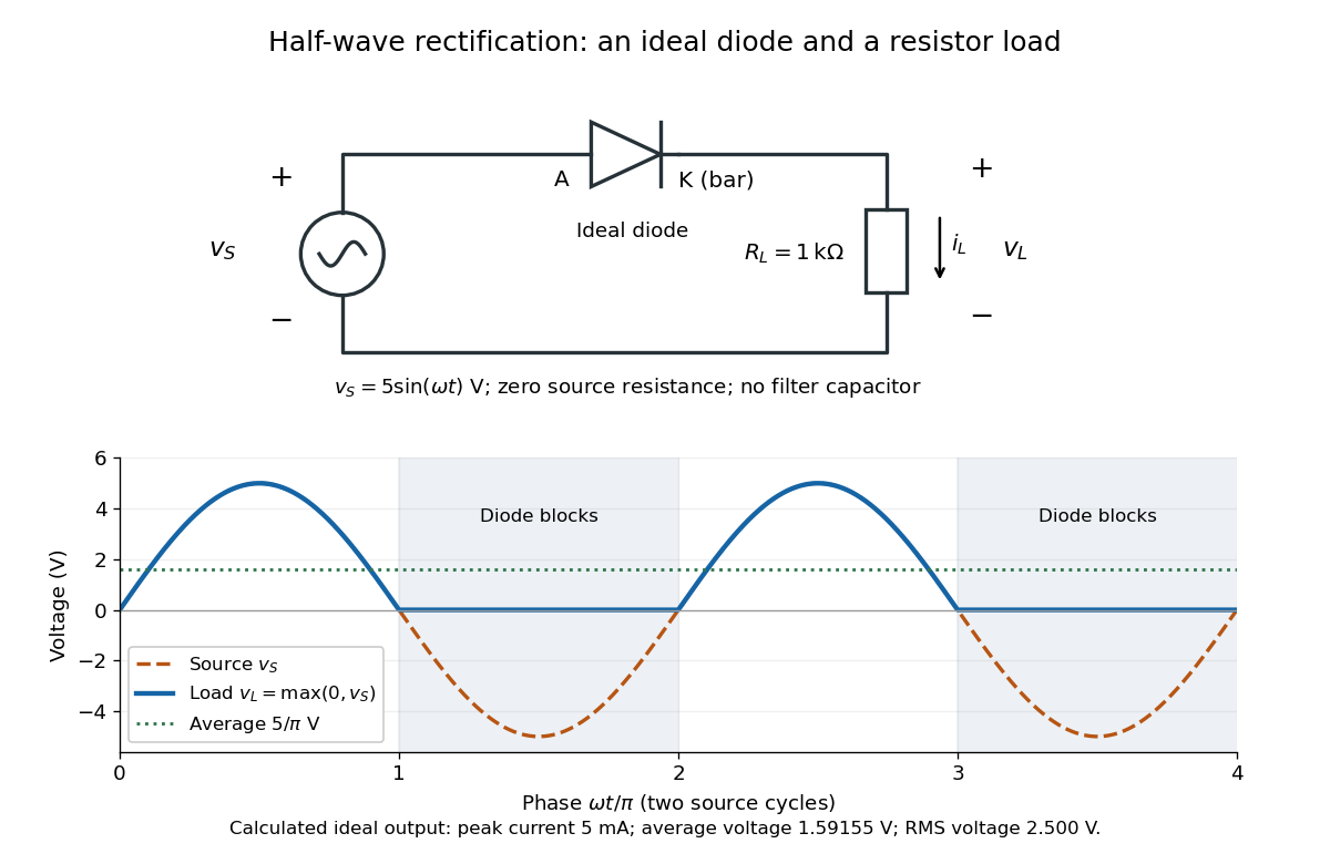
An ideal half-wave rectifier selects the positive half-cycle
. Original schematic and calculated load electric potential difference for and . The diode cathode is the bar at ; positive load electric current flows downward through the resistor. Dashed orange: source sinusoid. Blue: load output, zero during the negative half-cycle. Green: its cycle-average electric potential difference . No smoothing capacitor is present; these are ideal model predictions. Details.
The Kirchhoff cycle law gives , and Ohm's law gives . If , the blocking assumption would give , contradicting the ideal diode model, so the diode conducts with . If , conduction would give , also forbidden, so the diode blocks. At the crossings both values vanish. ThusThe peak load electric current is . The output is unidirectional but still varies in time, reaching zero throughout every negative half-cycle. Over a period of a function , write the wave phase as . Its average value of a function and root mean square follow from two integrals:Consequently the average load power is , not . The ideal diode has zero loss; the resistor converts supplied energy into Joule heating. The same switching argument predicts when the diode is reversed. Directional selection changes the waveform and its average value of a function; it does not by itself produce a constant output.
Voltage multiplier 2026-10-18
An electrical circuit that uses diodes and capacitors to produce an output electric potential difference larger in magnitude than the input peak. The attainable output depends on the circuit arrangement, electric current drawn by the load, capacitance and input frequency; an ideal unloaded result does not specify the output under load.
Lens bound on a reconstructed Fermi pocket 2026-10-18
In rectangular-lattice Fermi-surface reconstruction, the zero-coupling closed orbit is the overlap lens of two equal circles of radius with centres separated by . Two circular sectors minus their triangular portions giveAt fixed chemical potential, the upper hybridized energy band rises when the magnitude of the Fourier coefficient increases. Its occupied pocket therefore shrinks, so this lens is an upper bound in the two-wave model. It is not a universal bound for arbitrary changes of chemical potential or additional energy bands.
Put , , , and . The upper eigenvalue of the two coupled plane waves isAt fixed Fermi energy , its closed Fermi contour hasThus can be inverted numerically to estimate the Bragg scattering coupling. The pocket disappears at . The estimate assumes a fixed chemical potential and neglects coupling to other plane waves; a measured pocket area alone does not determine all Fourier coefficients of an arbitrary lattice potential.
2001 attosecond pulse-train experiment 2026-10-18
Pierre Agostini's experiment illuminated an argon jet with an annular beam. A pinhole removed the annulus; a tungsten-coated mirror relayed harmonics and weak central reference into another argon jet. A magnetic-bottle electron spectrometer used time of flight and microchannel plate detectors. Glass plates varied delay. Reference-on sidebands contrasted with reference-off peaks. Atomic-phase-corrected reconstruction yielded -attosecond bursts.[ref]
Observation of a Train of Attosecond Pulses from High Harmonic Generation by P. M. Paul and others. pp.1690–1691, Figs.1–4 and Table 1
The two-path attosecond phase reconstruction explains the control's purpose: adding the reference opens an interference channel. Its fitted oscillation tests phase relationships under the weak-field and atomic-response model. It does not independently reveal every target phase or an arbitrary nonperiodic optical pulse.
Two-path attosecond phase reconstruction 2026-10-18
An original two-amplitude model makes the timing inference explicit. Use the spectral phase convention of the coherent harmonic pulse-train model, and define positive delay to retard the reference electric field. Let the amplitudes leading to the same final photoelectron state bewith real . Squaring their sum givesThe oscillation comes from opposite signs of the reference photon's phase. For and , the signal peaks at modulo . A fitted phase contains the target contribution ; setting it to zero is an assumption, not an observation. In an experiment, unobserved final channels can add as probabilities, so the displayed formula is one effective-channel idealization.
For a chosen example, impose radians and radians at . The observed oscillation has argument . Its peak shift is , while the corrected finite-difference group delay is . Ignoring the target contribution would bias the inferred delay by attoseconds. These stipulated phases demonstrate a reconstruction error; they are not atomic calculations or measured delays.
Recovering all neighboring phase differences determines the component spectral phases up to an overall phase and the chosen timing origin, provided the oscillation phases are consistently unwrapped. Known component amplitudes then give a temporal field by a finite inverse Fourier transform. This is why measuring the optical spectrum alone is insufficient: it omits the very information that decides when constructive wave interference occurs.
For in a rectangular box with zero Dirichlet boundary conditions, separation of variables gives spatial eigenfunctions and temporal rates . The largest rate is the displayed one. Every nonzero nonnegative initial density has positive projection onto this first eigenfunction, so its sign determines eventual exponential growth or decay; equality leaves a stationary first mode. At fixed volume, write : their product is fixed, and the arithmetic-geometric mean inequality minimizes their sum when all three are equal. Thus the cube maximizes the growth rate among rectangular boxes of fixed volume; making a box sufficiently thin suppresses growth.
For nonnegative nonzero integrable initial data on , the first coefficient in the normalized Fourier sine series is strictly positive, because the first sine eigenfunction is positive throughout the interval. For with zero Dirichlet boundary conditions, the first decay rate is . Every higher rate exceeds it by , so smoothing for positive time and the spectral gap imply uniformly. Thus all interior points share the growth/decay threshold ; the endpoints remain zero. At equality the limiting profile is nonzero and stationary.
Removing a variable scalar reaction rate by an integrating factor Created 2026-10-18 Updated 2026-10-20
For , the displayed substitution converts the equation exactly into the heat equation . The scalar prefactor preserves homogeneous Dirichlet boundary conditions. Consequently each spatial eigenfunction with acquires temporal factor . The same algebra works with an evolution variable named ; calling that variable spatial does not alter the separation of variables. For , the prefactor normalized to one at zero is .
For on with , , and , the Rayleigh quotient is . The trial gives numerator and denominator , hence . Every displayed obeys the same mixed boundary conditions; so does . Adding any of these to the trial space cannot worsen the optimized upper bound. Matrix elements and give a finite-dimensional generalized eigenvalue problem . The case repeats the original trial and adds no variational freedom.
Affine-parameter Sturm-Liouville eigenvalue bound Created 2026-10-18 Updated 2026-10-20
For a self-adjoint Sturm-Liouville operator with common boundary conditions and an -normalized lowest eigenfunction of , evaluating the Rayleigh quotient on gives the displayed upper bound. More generally the lowest eigenvalue is the infimum of affine functions of , so it is concave in that parameter. The trial state must satisfy the boundary requirements of the variational domain; changing the operator without changing the trial function's normalization can still be legitimate when the weight is fixed.
Ultraviolet catastrophe 2026-10-18
The ultraviolet catastrophe is the divergent total thermal radiation energy predicted by classical equipartition theorem applied to the electromagnetic mode density in a box. Each mode has mean energy , while the number of modes per volume per frequency is . The Rayleigh-Jeans law therefore gives , whose integral over all positive frequencies diverges at every .
Planck's law replaces the classical mode energy by . It agrees with equipartition when but suppresses high-frequency excitations exponentially. The resulting spectral energy density is integrable and yields the finite Stefan–Boltzmann law. The failure concerns the classical equilibrium distribution of energy among modes, not the existence of electromagnetic wave propagation itself.
Outgoing longwave radiation 2026-10-18
Outgoing longwave radiation is the outward thermal radiative flux at the top of the atmosphere, integrated over the specified thermal spectrum and outward directions. It differs from a directional spectral radiance.
Convective adjustment Created 2026-10-18 Updated 2026-10-25
Convective adjustment replaces an excessively steep vertical temperature gradient by an allowed profile while respecting the selected energy budget. It is a closure for unresolved convection, not a direct simulation of individual rising parcels. A prescribed critical atmospheric lapse rate is a modeling assumption; it need not equal the dry adiabatic lapse rate.
For an original dry two-slab example, take fixed equal heat capacities and slab centers separated by . Initially below and above. Stipulate a permitted atmospheric lapse rate . The initial difference exceeds the allowed . Conservation of the sum of the two sensible energies requires , while the adjusted gradient requires . Hence and . Heat removed below equals heat added above. Simply holding the lower slab fixed and raising the upper slab to would introduce external energy.
For unequal constant heat capacities , the same two constraints instead giveApply this adjustment only when the original gradient exceeds the threshold. A moist adjustment also has to account for latent heat and changing composition; conservation of this dry sensible-energy expression alone is then insufficient.
For a fixed circular elastic membrane, the Rayleigh-Ritz variational principle applied to , , gives . The numerator of its Rayleigh quotient is , and the denominator is . Minimization gives , , and the displayed upper bound for the ordinary frequency . Every has finite radial Dirichlet energy, which is the required variational admissibility condition.
Radial reduction and growth at infinity 2026-10-18
For , the substitution removes the first derivative in the three-dimensional radial Laplacian, since . Bounded at zero implies . Bounded at infinity means ; it does not require bounded . For example, constant forcing has the bounded particular solution , whose reduced function is . A Dirichlet half-line Green function for d2 minus 1 can still represent this solution when its integral converges, but the resulting reduced function has the growth demanded by the forcing.
Lamé stress distribution in a pressurized cylindrical wall Created 2026-10-18 Updated 2026-11-05
For inner and outer radii , with internal and external pressures , the boundary tractions are and . The radial equilibrium of a thick elastic cylinder gives and . The radial compressive pressure is . Since hoop stress is monotone in when , its maximum absolute value is the larger of and . With negligible external pressure, its maximum is the tensile inner-wall value . The stress distribution itself is independent of elastic moduli in this linear homogeneous axisymmetric model; its associated displacement depends on them.
Character table of the quaternion group 2026-10-18
The quaternion group has conjugacy classes , , , , , with sizes . Over the complex numbers, the number of classes and the sum of squares of irreducible representation dimensions force four one-dimensional representations and one two-dimensional representation. For , the linear character rows on these classes are . Orthogonality then gives the remaining row . A representation with character contains two copies of the two-dimensional irrep and none of the linear irreps, by the character inner product. The choice of scalar field matters: the corresponding quaternionic four-dimensional real representation is irreducible over the reals.
Quaternion group modulo its centre 2026-10-18
In the quaternion group, commutes with each generator because any element commutes with its powers. Hence is central and is a normal subgroup. The reverse products satisfy , , , so none of is central. Therefore .
The four cosets are . Each nonidentity coset squares to , and . Thus the quotient group is the Klein four-group. Explicitly, mapping to its identity and mapping to its three different nonidentity elements is a surjective group homomorphism with group kernel . The first isomorphism theorem gives the title result.
There are unlisted articles, also show them or only show them.