
Vapor-liquid equilibrium Created 2026-10-18 Updated 2026-11-05
Vapor-liquid equilibrium is coexistence of a liquid and its vapor with no net macroscopic transfer of matter between them. The two phases have equal temperature, equal pressure for a flat interface without external stress, and equal chemical potential for each exchanging species.
For a pure substance, fixing the temperature below its liquid-gas critical point selects the saturation vapor pressure. Molecules still cross the interface in both directions; equilibrium means equal average opposing rates, rather than halted molecular motion. In a mixture, the vapor and liquid generally have different compositions, while each component separately satisfies the chemical-potential equality. This distinction underlies separation by evaporation and condensation and explains why equal total pressure alone is insufficient to determine phase compositions.
Magnetron motion 2026-10-18
The slow radial normal mode of a Penning trap. Its angular frequency arises from the combined static electric field and magnetic field; it is distinct from the driven Paul trap micromotion.
Kelvin thermoelectric relation 2026-10-18
With the Seebeck coefficient convention at zero electric current, and the transported-heat convention of Peltier coefficient, the Kelvin thermoelectric relation is is absolute temperature in kelvins; use consistent material references. This scalar linear response relation assumes local thermal equilibrium and reciprocal transport without time-reversal-breaking fields or order. Onsager reciprocal relations supply the symmetry; conservation of energy alone is insufficient. A magnetic field requires a reversed-field reciprocity comparison.[ref]
In particular, the A-minus-B thermocouple coefficient in Seebeck effect is , whereas absorbed junction heat for conventional current A to B uses . There is no contradiction: terminal voltage order and crossing direction are separate choices. Multiplying a measured voltage by an absolute temperature without specifying these choices does not determine junction heating.
A short reciprocity calculation makes the factor visible. At a common reference temperature, write the local linear response with electrical driving field and heat flux asAt , the Seebeck coefficient convention gives . At , the Peltier coefficient is . Thus gives . The chosen forces are conjugate to the fluxes in the local entropy production, ; arbitrary rescaling of just one force would spoil this argument.
The relation is local. Varying permits distributed Thomson effect heating, with ; the constant-coefficient model below omits it. Endpoint substitutions into a constant-property formula can therefore break its energy accounting.
Redshifting of peculiar momentum 2026-10-18
A freely moving massive test particle in an FLRW metric has physical momentum relative to a comoving observer, where is its peculiar velocity. For a radial geodesic, the geodesic Lagrangian gives constant, and the local radial momentum is . The proper-time normalization gives , soConsequently nonrelativistic peculiar velocity scales as , while the exact relativistic law keeps . The momentum magnitude of a free photon also scales as , giving cosmological redshift through . These statements concern force-free propagation; a bound system need not follow the cosmological expansion.
Paul trap secular-motion example 2026-10-18
Choose these dimensionless parameters for an original example, with no collisions or damping. They are teaching inputs, not measurements from either lecture. With and slow initial amplitude , the radial equation and its leading approximation areSet and to match the approximate initial conditions. The leading secular angular frequency is . The velocity Verlet method integrates the full RF equation over 80 drive periods; a separate fourth-order Runge-Kutta method checks the computed trajectory. Halving the timestep tests numerical error independently of the averaging error.
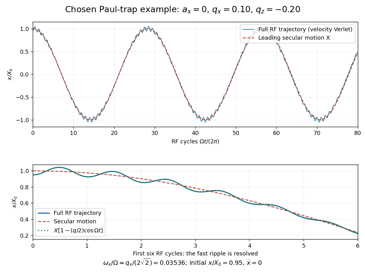
Full RF motion and the leading secular approximation
. Original chosen small-parameter calculation in units of . The lower panel resolves six drive cycles and includes the first micromotion correction. Agreement over this finite interval does not establish a stability diagram or an exact secular frequency. Details.
Using 400, 800, 1600 and 3200 steps per RF period gives successive maximum position differences of approximately , and in units of , consistent with second-order convergence. The finest trajectory differs from the independent classical fourth-order Runge-Kutta method result by at most , whereas differs by as much as . Over a sufficiently long time, the omitted correction to the secular angular frequency produces a growing phase discrepancy even if the numerical trajectory has converged. For the chosen point only, integration of a fundamental solution matrix over one RF period checks that both the radial and axial Floquet multipliers lie on the unit circle, away from its endpoints. This tests simultaneous ideal confinement without extrapolating to larger .
Polarized beta-decay angular distribution Created 2026-10-18 Updated 2026-10-20
Consider a parent atomic nucleus at rest. Write its signed nuclear polarization along a fixed axis as , where is its maximal spin component. Let be the angle of the emitted electron momentum to that axis and let . Use for the parity operator, so it is not confused with .
For an axially symmetric leading-dipole model, retain a constant and the term linear in the polarization vector . Rotational symmetry makes the directional term proportional to . Define its dimensionless coefficient as . At fixed electron energy the relative intensity and normalized probability density function per solid angle are thereforeThe factor is the conventional separation of the speed dependence; rotational symmetry alone does not determine that dependence or . The coefficient contains the decay dynamics. This leading model omits higher angular terms and detailed recoil and radiative effects. A partially oriented higher-spin ensemble can also have alignment that is not specified by its vector nuclear polarization alone.
The unit-integral condition follows without any model of a detector:Thus has unit angular average, while the probability density function in the polar angle alone contains the Jacobian determinant factor:In particular, itself is neither a normalized probability density function in nor a detector count. Positivity on gives .
Under full spatial reflection, but . The latter follows already for orbital angular momentum from ; spin has the same axial vector transformation. Hence is a pseudoscalar, and . If parity conservation held for this model, equal probabilities for the inverted process would force . Conversely, in an unpolarized sample proves nothing about .
Integrating over the two hemispheres gives a useful original check:Choose , , and , so . Then the forward and backward hemisphere probabilities are and , and their counting asymmetry is . These are chosen teaching values, not measured values from the Wu experiment. At a single energy, the angular shape determines the product ; it cannot separately determine without a polarization calibration.
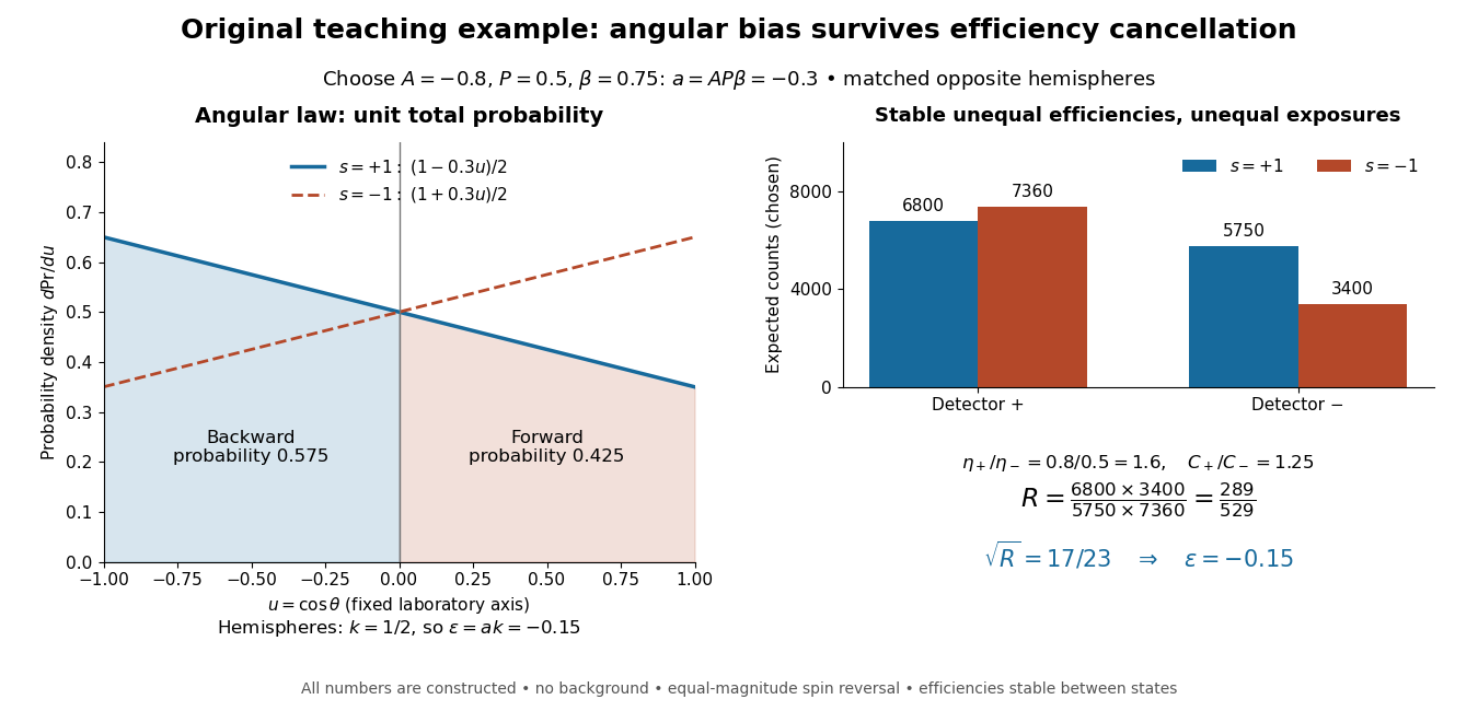
Chosen angular probabilities and detector-efficiency cancellation
. Original model with . The angular probability is distinct from a detector count; opposite hemispheres average the cosine to . Unequal efficiencies and exposures distort individual detector ratios, while a reversal cross-ratio recovers the chosen hemispheric asymmetry. All counts are constructed. Details.
Wu experiment Created 2026-10-18 Updated 2026-10-20
The Wu experiment was performed by Chien-Shiung Wu, Ernest Ambler, Raymond Webster Hayward, Dale D. Hoppes, and Ralph Percy Hudson; its 1957 report was Experimental Test of Parity Conservation in Beta Decay. Their experiment supplied the evidence that the Lee-Yang proposal for a parity test had called for.[ref]
The Fall of Parity Photo Gallery with Short Biographies by National Institute of Standards and Technology. Experimentalists: the five named biographies; theorists: Lee and Yang
A cobalt-60 surface layer on a cerium magnesium nitrate crystal was cooled by adiabatic demagnetization; a solenoid's magnetic field polarized its atomic nuclei. An internal anthracene counter detected electrons by particle scintillation; a light pipe carried flashes to a photomultiplier. Polar and equatorial gamma ray counters monitored nuclear polarization and effective temperature; bulk thermometry could miss surface heating.[ref]
Experimental Test of Parity Conservation in Beta Decay by Chien-Shiung Wu and others. p. 1413, Fig. 1 and apparatus paragraphs; p. 1414, demagnetization followed by vertical solenoid
Reversing nuclear polarization reversed the electron excess; warming erased it with gamma ray anisotropy. Warm rates were field-independent. Cooling-field reversal checked remanence; poorly polarized sources checked magnetic deflection. Electrons favored the direction opposite spin.[ref]
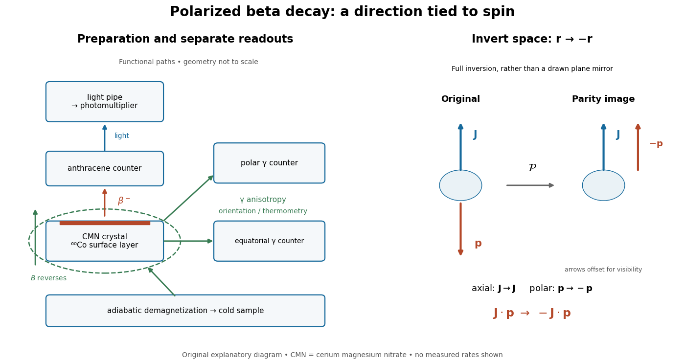
What the apparatus measures, and what spatial inversion changes
. Functional layout, with paths separated for readability. The right-hand construction inverts every spatial coordinate: a polar momentum reverses while an axial spin remains fixed. It is a geometric argument, not a second historical apparatus. Details.
The gamma ray anisotropy diagnoses the preparation; the electron asymmetry diagnoses parity violation. These are different jobs. A directionally uneven gamma ray signal alone need not violate parity conservation: a distribution even in the cosine of the angle can distinguish an axis from its perpendicular without distinguishing its two ends. The spin-momentum correlation instead distinguishes those ends.
The inference requires control of changes in detection efficiency, electron transport and nuclear polarization. A fixed detector under spin reversal avoids physically exchanging detector positions, but still requires checks for magnetic field effects. The result establishes parity violation in this weak interaction process. A precise microscopic coupling requires more information than the existence or sign of a counting asymmetry; the following model makes that distinction explicit.
Lee-Yang proposal for a parity test Created 2026-10-18 Updated 2026-10-25
In 1956, Tsung-Dao Lee and Chen Ning Yang examined the evidence for parity conservation in the weak interaction. Their paper, Question of Parity Conservation in Weak Interactions, distinguished an untested assumption from an established experimental result and proposed comparing electron emission along opposite directions relative to oriented nuclear spins, explicitly considering cobalt-60. It proposed a test; it did not report the later Wu experiment.[ref]
Question of Parity Conservation in Weak Interactions by Tsung-Dao Lee and Chen Ning Yang. pp. 254–255; evidence review and “Possible Experimental Tests of Parity Conservation in beta Decays,” first proposal
The conceptual improvement is the choice of observable. An angle between two polar vectors is preserved by spatial reflection; its distribution can conceal parity violation. An angle between an axial vector and a polar vector changes to its supplement. Thus a spin-resolved directional measurement asks a different question from an unpolarized total decay rate.
Spin-one-half paramagnetic magnetization Created 2026-10-18 Updated 2026-11-05
Curie–Weiss law Created 2026-10-18 Updated 2026-11-05
The Curie–Weiss law approximates the magnetic susceptibility of interacting localized moments by in a suitable paramagnetic temperature range. A positive Weiss temperature often reflects predominantly ferromagnetic interactions, while a negative value often reflects antiferromagnetic interactions. It is not a universal exact law through an ordering transition, and crystal-field effects or itinerant carriers can require another description.
Rectangular parallelepiped Created 2026-10-18 Updated 2026-10-20
A rectangular parallelepiped is a parallelepiped whose three edge directions at each vertex are mutually perpendicular. Its faces are rectangles; if its edge lengths are , its volume is . A cube is the special case .
Vertex of a parabola 2026-10-18
For a parabola described by the function graph , with nonzero in the real numbers, its vertex of a parabola is the point . This point gives its minimum or maximum value of in these coordinates.
For the upper half-space and the sign convention , reflect the source to and use the displayed difference. This is the negative of the conventional outgoing kernel, whose source sign is . The method of images makes the Dirichlet boundary condition zero on the plane. With and , its outward normal derivative there isThe outward unit normal is . Differentiating gives ; the real and reflected source contributions add in the normal derivative. Green's second identity therefore expresses a solution of the Helmholtz equation as when the boundary term at infinity vanishes. Suitable decay or compatible outgoing Sommerfeld radiation conditions are needed; vanishing at infinity without further control is not a general uniqueness condition for a real-frequency Helmholtz problem.
For , and the convention , the spatial Fourier transform gives the multiplier . Aligning the Fourier polar axis with gives and hence the displayed radial integral.
The pole on the integration path requires a prescription. The Cauchy principal value gives . The outgoing prescription is , yielding ; the opposite prescription gives the incoming exponential. The Sokhotski–Plemelj formula shows that the additional radial contribution is .
Let for , with real , and uniformly in direction. With sufficient boundary regularity, Green's second identity on an expanding half-ball gives the title formula. The plane integral is interpreted as the limit over expanding disks when it is not absolutely convergent. Its sign uses the upward derivative ; the outward normal derivative is .
For , and at large . The hemispherical integrand can be written , whose integral tends to zero by the Sommerfeld radiation condition. Add the boundary identities for a source point and its reflected point . On the plane and their normal derivatives are opposite. The terms involving boundary values of cancel, leaving twice and hence the title formula. In particular, zero Neumann boundary data imply in this radiating class.
Orthogonal involutions of the plane Created 2026-10-18 Updated 2026-11-05
For a real orthogonal involution, , so it is a symmetric matrix. Its eigenvalues are . In two dimensions the possibilities are the identity, the half-turn , and reflectionsThe reflection fixes the line making angle with the first coordinate axis and negates its perpendicular direction. This follows either from the two corresponding eigenvectors or by rotating . A nonidentity element of order two in a faithful representation must be either the half-turn or a reflection; the identity matrix is excluded by faithfulness.
Radial-velocity semi-amplitude 2026-10-18
Half the full range of an orbit-induced line-of-sight velocity variation, after accounting for a constant systemic offset.
Comb tooth index ambiguity 2026-10-18
One beat magnitude does not tell us the integer . In the example, every proposed optical frequency produces the same signed beat with its corresponding tooth. A coarse independent optical measurement can select the integer: once the beat sign is known, an error bound below suffices if the candidate is selected by nearest distance.
There is also a useful two-spacing check. Keep the unknown laser and fixed, track the same tooth continuously, and increase by a stipulated . Its frequency rises by , so the signed beat falls from to . HenceThis inference fails if the unknown drifts appreciably, the offset changes unnoticed, the beat sign is lost, or the tracker jumps to another tooth. The assumed tooth motion stays well below half the spacing in this example. If also changes by a measured amount, use .
For a fixed verified tooth number, the first-order frequency error is . Errors in these readings can be correlated because they share a reference. A small beat uncertainty therefore does not imply the same absolute optical accuracy: the reference's calibration and the factor remain in the error budget. A wrong tooth number is a separate discrete error, not a small correction. The beauty of the comb is that two controlled parameters organize millions of optical reference points, while the unknown's position is read electronically.
Optical fiber cutback measurement 2026-10-18
An optical fiber cutback measurement estimates distributed optical fiber attenuation by comparing a long guide with the short input portion left after cutting the output end back. Keep the launch untouched. For the following original functional model, fix wavelength, source output, input alignment and collected output cone; subtract a dark reading and keep the photodetector in its linear range. Renewed end-face quality and changed normal mode populations can still spoil the comparison. The diagram describes a measurement principle, not Kao's historical short-glass apparatus.
Let be lengths in kilometres, the corresponding positive dark-subtracted readings, and the same launch and detection factor. A uniform guide obeysHere and its estimate are numerical values in . Dividing eliminates ; taking a logarithm proves the formula. A changed instead adds an error . Reconnecting the launch between readings defeats this cancellation.
For original chosen values , , and , the predicted long reading is . The ratio gives for the removed and hence .
Suppose an unremoved additive detector background contributes to both readings. Then the apparent coefficient isThis is a bias of an estimator: a common additive background pushes the ratio toward one, whereas a common multiplicative factor cancels. For independent small zero-mean errors with standard deviations on the dark-subtracted readings, a first-order Taylor expansion givesChoosing both standard deviations as gives . A shared estimated dark offset introduces covariance, so it requires a different uncertainty calculation. Near zero signal, the logarithm and this linear approximation become unreliable.
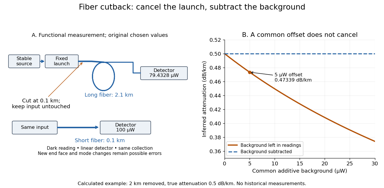
Optical fiber cutback measurement: fixed launch and additive-background bias
. Original functional schematic and calculated example. The launch stays fixed while the remote end is cut back. The graph uses the stipulated powers and lengths above; it compares dark-subtracted readings with a common positive unremoved background. No plotted point is a historical measurement. Details.
Ideal operational amplifier 2026-10-18
An ideal operational amplifier has infinite open-loop gain and input impedance, zero output impedance, unlimited response speed and zero input offset voltage and input bias current. Its input currents vanish. In a stable linear circuit with negative feedback and a finite output, its differential input voltage tends to zero as the open-loop gain tends to infinity. Thus and are the familiar conditional circuit rules. The equality of the input voltages cannot be imposed on an open-loop, unstable or saturated circuit.
There are unlisted articles, also show them or only show them.