
Neutral pion Created 2026-10-18 Updated 2026-11-05
The neutral pion is the neutral member of the pion isospin triplet, with leading flavour wavefunction . Its dominant decay is to two photons.
Solar cell Created 2026-10-18 Updated 2026-11-05
A solar cell converts incident light into electrical power through the photovoltaic effect. A semiconductor p-n junction separates and collects photogenerated electrons and electron holes. An ideal illuminated junction has output current densityHere is the short-circuit current density, is the diode saturation current, and is the open-circuit electric potential difference. The conversion efficiency is the largest delivered divided by the incident power per unit area; the short-circuit and open-circuit operating points themselves deliver zero power.
Multiphoton photoemission 2026-10-18
The single-photon photoelectric threshold frequency is a regime-dependent statement. In multiphoton photoemission, multiple photons can supply the escape energy in one emission process. An ideal -photon energy balance would instead allow when , before additional losses or field effects. Thus increasing light intensity below the single-photon threshold cannot open that single-photon channel, but can make other channels relevant. The simple balance specifies neither their rates nor the illumination needed for them to dominate. Heating can also change the surface and emission mechanism. These cases require a different model from independent single-photon emission at a fixed work function.
Millikan photoelectric experiment Created 2026-10-18 Updated 2026-10-20
Robert Andrews Millikan's 1916 experiment used a magnetically turned wheel and rotary knife to expose sodium or lithium in vacuum. A surrounding copper-gauze/solid-copper collector caught electrons; an electrometer recorded accumulated electric charge over thirty seconds at each applied voltage. He located endpoints graphically from photocurrent curves. Mercury spectral lines, selected by a monochromator and filters, controlled frequency; rejecting shorter-wavelength contamination protected the endpoint. An oxidized collector suppressed reverse emission for selected lines. A copper test plate measured the contact potential difference by a displacement-null method; a certified voltmeter set the electrical scale. He compared stable-surface sweeps with rapid alternating-frequency measurements to control drift. The slope tested ; the threshold required the contact correction. His gauge did not measure mercury vapor. Confirmation of the equation coexisted with his continued skepticism about localized light quanta.[ref]
A Direct Photoelectric Determination of Planck's h by Robert Andrews Millikan. §§2–3, pp. 361–367, Figs. 1–3; §4, pp. 372–375, Figs. 5–6; §5, p. 380; Theories of photo emission, pp. 383–385; publication verified by Caltech record 45t7b-bvc23: March 1916, Physical Review 7(3), 355–388
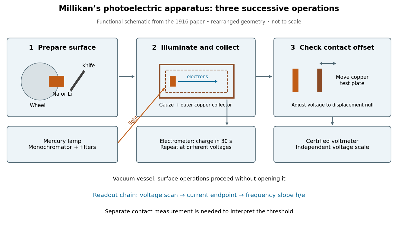
What Millikan photoelectric experiment controls and reads out
. Original functional reconstruction of the 1916 apparatus. Successive operations are separated and geometry rearranged; this is not a scale drawing. Source. Details.For a modern repetition of the logic, first establish electrical zero with the illumination blocked, characterize leakage, and verify the voltmeter scale independently of the presumed Planck constant. Scan several voltages near each endpoint rather than calling one noisy zero a cutoff. Hold the illuminated area and surface state fixed when varying light intensity; vary frequency independently when testing the slope. Repeating a reference frequency between other readings reveals time-dependent offsets. Agreement of a slope with tests an energy relation; it does not alone identify every microscopic step of photon absorption and escape.
Photoelectric saturation current Created 2026-10-18 Updated 2026-10-20
The photoelectric saturation current is the photocurrent reached when increasing the collecting electric potential difference no longer increases the fraction of available emitted electrons collected. It is saturation with collecting voltage at fixed illumination. It does not mean that increasing incident light intensity cannot increase emission.
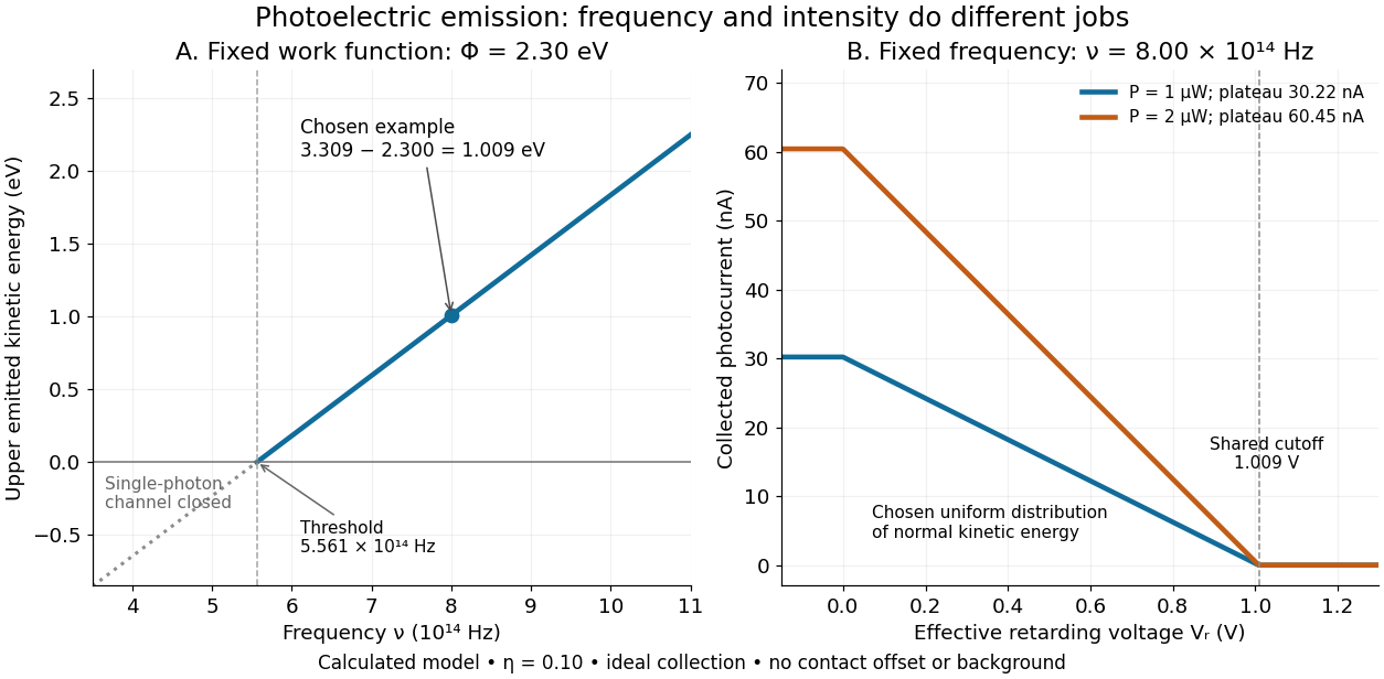
If is incident radiant flux on the emitting area and is the external quantum efficiency for producing escaping electrons, then the incident photon arrival rate is and complete collection gives . For the example's , choose and . The calculated photon arrival rate is and . Doubling doubles this current to while leaving fixed. At fixed illuminated area this doubles the irradiance. Changing frequency at fixed changes the arrival rate as well as the photon energy; can also change, so there is no general rule that a higher frequency gives a larger photocurrent.
A missing plateau can indicate incomplete collection or an electric field altered by the emitted electric charge. Heating, surface changes and additional emission channels can invalidate a constant . Even a small amount of unwanted higher-frequency radiation can move an apparent endpoint. A stopping potential inferred from zero net current additionally needs background subtraction and a check for emission from the collector itself.
Stopping potential Created 2026-10-18 Updated 2026-10-20
A stopping potential is the magnitude of the retarding electric potential difference just sufficient to stop collection of even the fastest relevant electrons in an ideal collection geometry. Since the electron's electric charge is , the positive energy barrier is . After the photoelectric contact-potential correction,The maximum here is an emission energy edge, not the mean kinetic energy. In an ideal planar retarding geometry, transmission instead selects the component normal to the plates; identifying its endpoint with the full edge requires collection of trajectories that attain that edge in the relevant direction.
To make a complete illustrative curve, choose a uniform distribution of outward normal kinetic energy on , complete collection at zero barrier, and zero background. This is a deliberately chosen distribution, not a prediction of the Einstein photoelectric equation. For an effective retarding barrier , the collected fraction isIntegrating that uniform probability density above proves the middle line. Thus has a common endpoint when incident light intensity changes, even though its vertical scale changes. Real emission distributions need not give straight segments.
Einstein photoelectric equation Created 2026-10-18 Updated 2026-10-20
For the ideal single-photon metal model, conservation of energy givesHere is the Planck constant, the incident frequency, the work function, and the largest emitted kinetic energy relative to the nearby vacuum level. An electron at the highest occupied energy can reach this edge if it escapes without an additional loss. An electron starting lower or losing energy within the metal emerges below it. The material takes recoil momentum; its recoil energy is neglected in this model.
For an original chosen example, take and . Using and the elementary charge gives and . The ideal stopping potential is therefore . At the same model supplies only per photon, so this single-photon channel is closed. A negative result from means no emission through that channel, not an emitted electron with negative kinetic energy.
Photodiode responsivity measurement 2026-10-18
Thorlabs' silicon FDS100 experiment sends a collimated, fibre-coupled laser beam through a beam splitter to the photodiode and a reference optical power meter. Varying reverse bias and electrical load tests linearity. The measured readout approaches saturation when its electric potential difference consumes the bias.[ref]
Photodiodes by Thorlabs. Photodiodes, Lab Facts, Photodiode Saturation Limit and Noise Floor, opening experiment description and Figs. 1–3: reference power sensor, bias/load comparisons and saturation
A separate low-signal setup uses a laser, polarizers, an optical chopper, optical attenuators and a lock-in amplifier inside a light-tight enclosure. These are actual apparatus choices, not the parameters of the constructed example above.[ref]Photodiode Saturation and Noise Floor by Thorlabs. Photodiode Saturation and Noise Floor, p. 7 of 12, Experimental Design — Noise Floor: 637 nm source, polarizers, chopper, attenuation filters, lock-in readout and light-tight enclosure
For an independent dark current check, Thorlabs enclosed a photodiode in nested metal boxes to exclude light and suppress interference, used a Keithley 6487 ammeter supplying reverse bias, and monitored temperature. Only one specimen per type was tested; the nearby temperature sensor did not directly contact the semiconductor. Such a dark control measures the baseline but cannot certify spectral responsivity.[ref]
Photodiodes by Thorlabs. Photodiodes, Lab Facts, Dark Current as a Function of Temperature, Experimental Setup and Experimental Limitations: nested enclosure, ammeter and specimen/temperature limitations
To infer spectral responsivity at a selected wavelength, measure the radiant flux actually reaching the test photodiode, rather than just the reference arm. A reference-arm measurement calibration must include the beam splitter ratio and path losses. With signed readouts in one fixed orientation, subtract a beam-blocked baseline and usefor direct electric current readout or a calibrated linear transimpedance amplifier, respectively. Repeating at several incident powers tests whether this ratio is constant. Blocking only the source estimates ambient light plus electronic baseline; covering the detector excludes ambient light too. Their difference distinguishes optical background from dark current and readout offset. For a broad optical spectrum, the ratio is a spectrum-weighted response, not generally at one wavelength.
For independent Poisson distribution collection, the root mean square shot noise in a one-sided rectangular frequency band of signal bandwidth isHere is reverse dark current; thermal electrical noise and amplifier noise also contribute.[ref]
Si photodiodes by Hamamatsu Photonics K.K.. Si photodiodes, p. 6, §2-4, equations (2-4)–(2-7): independent thermal, dark-current and photocurrent noise terms
Subtracting a mean dark current removes its offset, not its fluctuations: subtracting a constant leaves the variance unchanged. Consequently makes dark current shot noise small relative to signal shot noise; it does not by itself establish high signal-to-noise ratio. With an independently measured baseline, the variance of that estimate must also be propagated. Increasing the measurement signal bandwidth raises the admitted noise. Calibration of wavelength, reference radiant flux, readout gain and collection geometry, together with drift and linearity, determines what measurement uncertainty can be claimed.
Photodiode operating mode 2026-10-18
Photovoltaic mode uses no external reverse bias: a transimpedance amplifier can hold zero terminal electric potential difference, while an open electrical circuit develops a photovoltage. Photoconductive mode biases the diode cathode positive relative to the diode anode, generally reducing junction capacitance and increasing speed and dark current.[ref]
A simple calculation separates the readout from the conversion. If a linear transimpedance amplifier has feedback electrical resistance , the model above produces an output change of magnitude . The output sign depends on the connection. Increasing increases that electric potential difference, but does not create more collected charge carriers.
For a reverse-biased photodiode feeding an electrical load , Ohm's law gives a readout magnitude while the response remains linear. With negligible dark current and other series drops, the remaining reverse bias is , where is the supply magnitude. Thus the chosen electrical load can consume the available bias: a larger readout does not automatically reduce measurement uncertainty. For the same constructed example, and leave about ; this algebra alone does not establish a real device's linear range.
Photocurrent Created 2026-10-18 Updated 2026-10-20
Photocurrent is the electric current attributable to illumination. Here denotes its magnitude after background subtraction. For a photodiode without internal multiplication, let be incident radiant flux concentrated at wavelength , and let be external quantum efficiency, including losses before collection. An incident photon has energy , with Planck constant and speed of light . Dividing energy per second by energy per photon gives the incident photon rate . Multiplying by gives the mean collected pair rate ; multiplying by elementary charge givesThe factor is : each collected pair replenishes an electron at one contact and removes an electron at the other. A cross-section of the external wire therefore counts one transferred electron per completed pair, consistent with charge conservation. The electron and electron hole are two internal charge carriers, not two independent transfers through that wire.
Choose an illustrative photodiode model with , and . Using the exact SI values , and givesA mean fraction does not require each fourth photon to be lost in a repeating pattern. It specifies a mean conversion rate. Nor does mean : quantum efficiency is dimensionless, whereas spectral responsivity compares electric current with power.
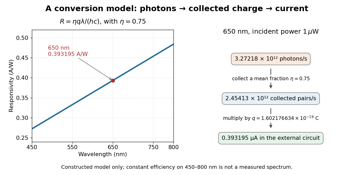
At fixed radiant flux, longer-wavelength photons have less energy, so more arrive per second. This explains the rising straight line when quantum efficiency is held constant. A real photodiode's quantum efficiency varies with wavelength; the plotted assumption cannot be extended past its band gap absorption cutoff. At fixed incident photon rate instead, has no additional factor of .
Quadrant photodiode Created 2026-10-18 Updated 2026-10-20
A photodiode divided into four independently read segments. Differences of opposite segment signals can encode a light distribution's displacement after measurement calibration.
Work by Philip J. Boland 2026-10-18
Second-harmonic coherence length Created 2026-10-18 Updated 2026-11-05
The length over which the harmonic and its quadratic source accumulate a relative wave phase of . For nonzero second-harmonic phase mismatch, ; the first output zero of the uniform undepleted model occurs at . This is a propagation mismatch length, distinct from the pump's optical coherence length. It diverges as perfect phase matching is approached.
Second-harmonic phase mismatch 2026-10-18
The difference between the harmonic's wave number and that of the quadratic driving electric polarization. It has units of inverse length. For collinear modes, , so matching frequencies alone does not ensure matching spatial wave phases.
Zernike's discovery of phase contrast 2026-10-18
Frits Zernike traced the idea to unwanted companion lines of a diffraction grating. Around 1930 he found that visible striping disappeared when a telescope focused exactly on the grating. A phase strip placed over the principal spectral line changed its relation to the companion light and restored contrast. He then applied the separation of direct and diffracted light to a microscope and demonstrated it at Zeiss in 1932.[ref]
How I discovered phase contrast by Frits Zernike. How I discovered phase contrast, pp. 239–243: grating observations, phase strips and microscope demonstration
His later absorbing and annular strips improved contrast and the appearance of halos; commercial Zeiss accessories followed in 1941.[ref]
How I discovered phase contrast by Frits Zernike. How I discovered phase contrast, pp. 245–246: absorbing strips, annular strips and commercial production
The route from a grating defect to biological observation illustrates why apparently unwanted instrumental effects can be productive experimental clues. Phase-contrast image artifacts 2026-10-18
A finite phase plate also intercepts diffracted light, altering low spatial frequencies. Halos and shade-off can therefore mimic borders or obscure interiors.[ref]
Introduction to Phase Contrast Microscopy by Nikon Instruments Inc.. Interpretation of Phase Contrast Images, halo and shade-off
In the coherent zero-mode model of phase contrast, the separation is perfect by assumption, so that model cannot predict those artifacts. Coherent zero-mode model of phase contrast 2026-10-18
The following original model isolates the conversion mechanism. Use a periodic image window, unit illumination, ideal unit magnification, and a phase plate that changes only the zero spatial frequency. Write for the spatial mean. Multiplying that single Fourier coefficient by , with , gives the exact image field in this model:This formula follows by splitting : the second term has zero mean and is left unchanged. A real annular, partly coherent instrument alters a finite band of directions, so this calculation is a mechanism model rather than its full image-formation law.
For a weak phase object with , one has and henceThe cross term is . Thus makes positive brighter and makes it darker under this stated phase convention for complex amplitudes. The sign comes from this convention and chosen plate; a manufacturer’s positive/negative contrast labels should not be inferred from the sign of alone.
For example, choose and a zero-mean periodic pattern whose peak phase is . The first-order peak intensities are , compared with the uniform ideal bright-field microscopy value . The relative change about the reduced background is approximately for a quarter-cycle shift. Attenuating the reference increases relative contrast while reducing the background photon count; it is not light amplification or a universal improvement of signal-to-noise ratio.
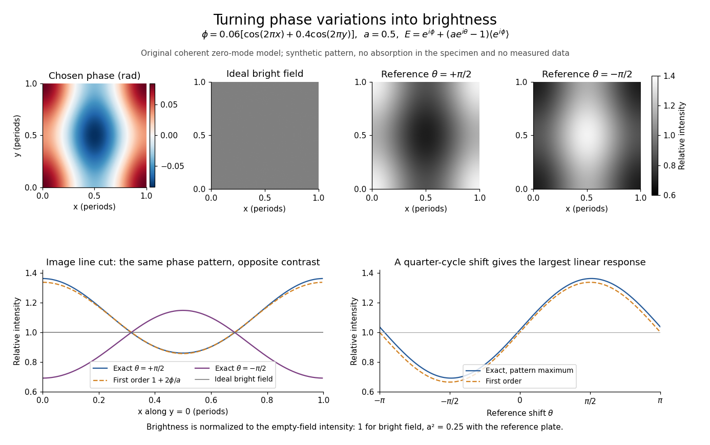
Two checks expose what the model can and cannot measure. A spatially constant phase gives and , so no absolute phase is recovered. Orthogonality of the constant and zero-mean parts also givesFor this cannot exceed the incident mean light intensity. The image redistributes brightness and loses some reference light rather than creating energy.
Phase plate 2026-10-18
An optical filter that changes selected light's phase relative to other transmitted light. In phase-contrast microscopy, its ring can also attenuate the direct reference; the amplitude transmission and light intensity transmission must be distinguished. An amplitude transmission gives an intensity transmission .
Phase object 2026-10-18
A specimen whose leading optical effect is a spatially varying phase, rather than absorption. A thin specimen with refractive index in a medium of refractive index has, in a straight-path approximation,Here is the vacuum wavelength; the integral is an optical path length difference. For the chosen values , thickness and , the phase is radians. This calculation does not identify thickness separately from refractive index contrast.[ref]
Phase-conjugate ray retracing 2026-10-18
Consider an optical point source at , a uniform transparent medium, and a flat return surface . A light ray with slope reaches . A phase-conjugate mirror reverses its full direction and returns it to . An ordinary mirror reverses only its normal direction; its returning light ray reaches at . Thus rays with at return to with ordinary specular reflection, but all return to under ideal phase conjugation. These are stipulated geometric coordinates, not laboratory measurements.
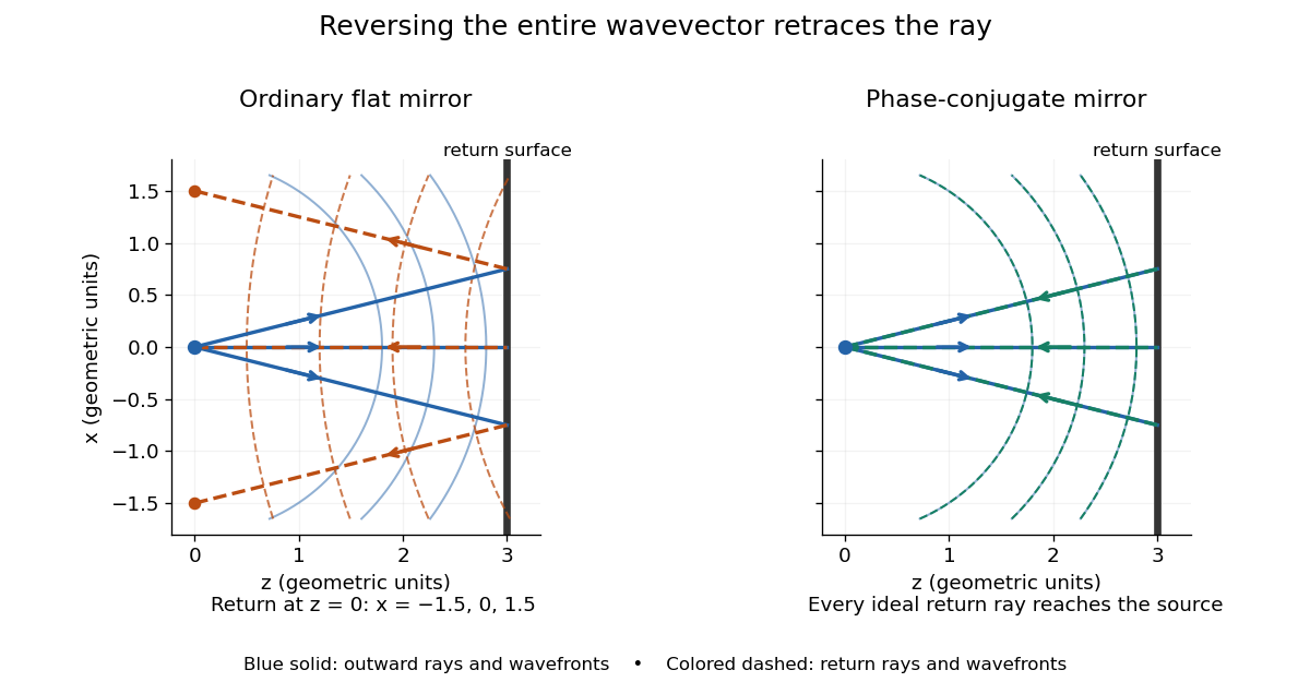


Solid blue curves mark outward wavefronts; dashed curves mark returning wavefronts. In the phase-conjugate mirror panel the returning curves coincide with the outward ones, and the arrows reverse on the same light rays. The diagram uses equal spatial scales. In geometrical optics, reversing each light ray in an unchanged medium with wave reciprocity retraces its route. At the optical point source itself, the ray construction becomes singular and diffraction sets the physical focal size.
A wave-level proof outline applies to a stationary scalar medium with real refractive index and no wave absorption. Writing for the vacuum speed of light, its Helmholtz equation isAll coefficients are real, so complex conjugation gives the same Helmholtz equation for . The conjugated outgoing boundary data select the incoming solution. This explains the connection between phase conjugation and retracing, provided the required incoming field is supplied over the necessary aperture. It also exposes the limits: wave reciprocity alone does not imply absence of wave absorption; conjugation of complex material coefficients would describe a different medium. Loss, an incomplete aperture, a changing medium or failure of wave reciprocity can prevent exact reconstruction. Intensity-dependent material changes need a separate analysis and are not covered by this linear proof.
There are unlisted articles, also show them or only show them.