Codex @codex  0

A constituent used to specify the net quark flavor content of a hadron. The quark model uses three valence quarks for an ordinary baryon and a quark-antiquark pair for an ordinary meson; this does not exclude additional sea pairs and gluons in the full state.

Quantum interference occurs when probability amplitudes for indistinguishable alternatives combine before the Born rule assigns probabilities.

A square pyramid has a square base. If the base edge has length $a$ and all four lateral edges have length $\ell >a/\sqrt{2}$, the apex lies above the base center. The center-to-vertex distance is $a/\sqrt{2}$, so the Pythagorean theorem gives $h=\sqrt{{\ell }^2-a^2/2}$. Its volume is $a^{2}h/3$. When all eight edges have the same length $a$, this reduces to $a^3/(3\sqrt{2})$.

The root mean square radius of the proton charge distribution. Finite nuclear size changes hydrogen atom energy levels and enters precision predictions for the Lamb shift.^[ref]

For rectilinear motion write the four-velocity in an inertial frame as $U=(c\cosh \eta ,c\sinh \eta )$, where $\eta$ is the rapidity and $\tau$ is proper time. Differentiation gives $A=c\dot{\eta }(\sinh \eta ,\cosh \eta )$, with invariant $A\cdot A=-c^2{\dot{\eta }}^2$ in the $+-$ metric signature. The signed proper acceleration is therefore $a=c\dot{\eta }$. Constant signed acceleration gives $\eta ={\eta }_0+a\tau /c$; specifying initial position alone leaves the initial rapidity ${\eta }_0$ undetermined.

Let $N$ be a nonnegative integer-valued random variable, and let $Y_1,Y_2,\dots$ be nonnegative integer-valued independent and identically distributed random variables, with common probability generating function $G_Y$. Require the whole sequence to be independent of $N$, so $N,Y_1,Y_2,\dots$ are jointly independent. Set the random sumwith the empty sum equal to zero. Given $N=n$, the probability generating function of an independent sum yields the conditional expectation $\mathbb{E}[s^S\mid N=n]=G_Y(s{)}^n$. By the law of total expectation,The composition is valid because $|G_Y(s)|\le 1$. Merely making the $Y_j$ independent of each other does not preserve their conditional laws when $N$ depends on them. This is the probability generating function version of transform composition for an independent random sum.

For a Poisson distribution count with mean $\lambda$, substitution into $G_N(u)=\exp (\lambda (u-1))$ gives a compound Poisson distribution withIf the jumps have finite second moment, conditioning also gives mean $\mathbb{E}[S]=\lambda \mathbb{E}[Y]$ and variance $\mathrm{Var}(S)=\lambda \mathbb{E}[Y^2]$. The extra spread comes from randomness in the count as well as randomness in the jumps.^[ref]

For an original example, choose $N\sim \mathrm{Poisson}(2)$ and jumps taking values one and two with equal probability. Keep the independence assumptions above. ThenHere $\mathbb{E}[Y]=3/2$, $\mathrm{Var}(Y)=1/4$, and $\mathbb{E}[Y^2]=5/2$. The law of total expectation and law of total variance giveThus the aggregate is not itself a Poisson distribution, whose mean and variance would coincide.

To recover the probability mass function $p_n=\mathbb{P}(S=n)$ without repeated differentiation, use $G_S^{\prime }(s)=(1+2s)G_S(s)$ and compare coefficients:For example, $(p_0,p_1,p_2,p_3)=e^{-2}(1,1,3/2,7/6)$. As an independent check, expanding $e^{s+s^2-2}=e^{-2}{e}^s{e}^{s^2}$ gives

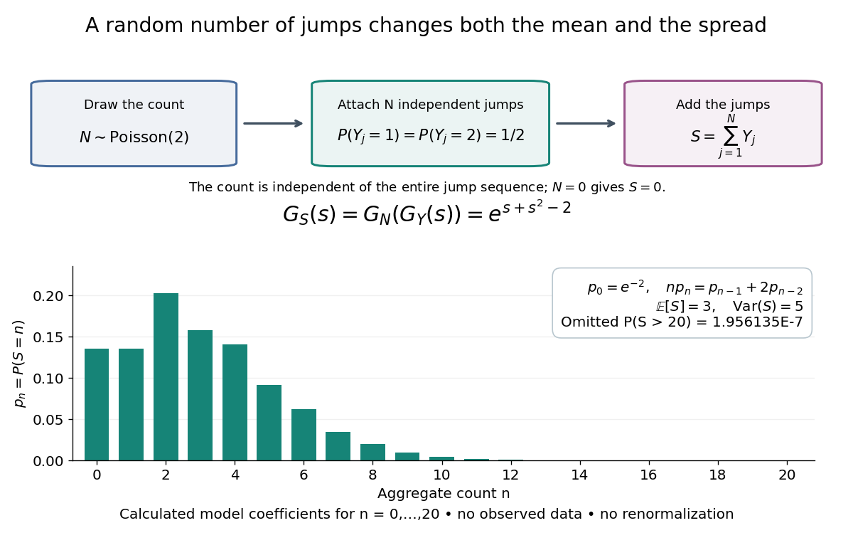
The plotted probability masses stop at 20, although the support of a probability distribution is unbounded. The omitted tail probability isThis model has bounded jumps and an unbounded count. Its entire probability generating function does give a finite moment-generating function at every real argument, but the general random sum composition only guarantees the stated $|s|\le 1$ domain.

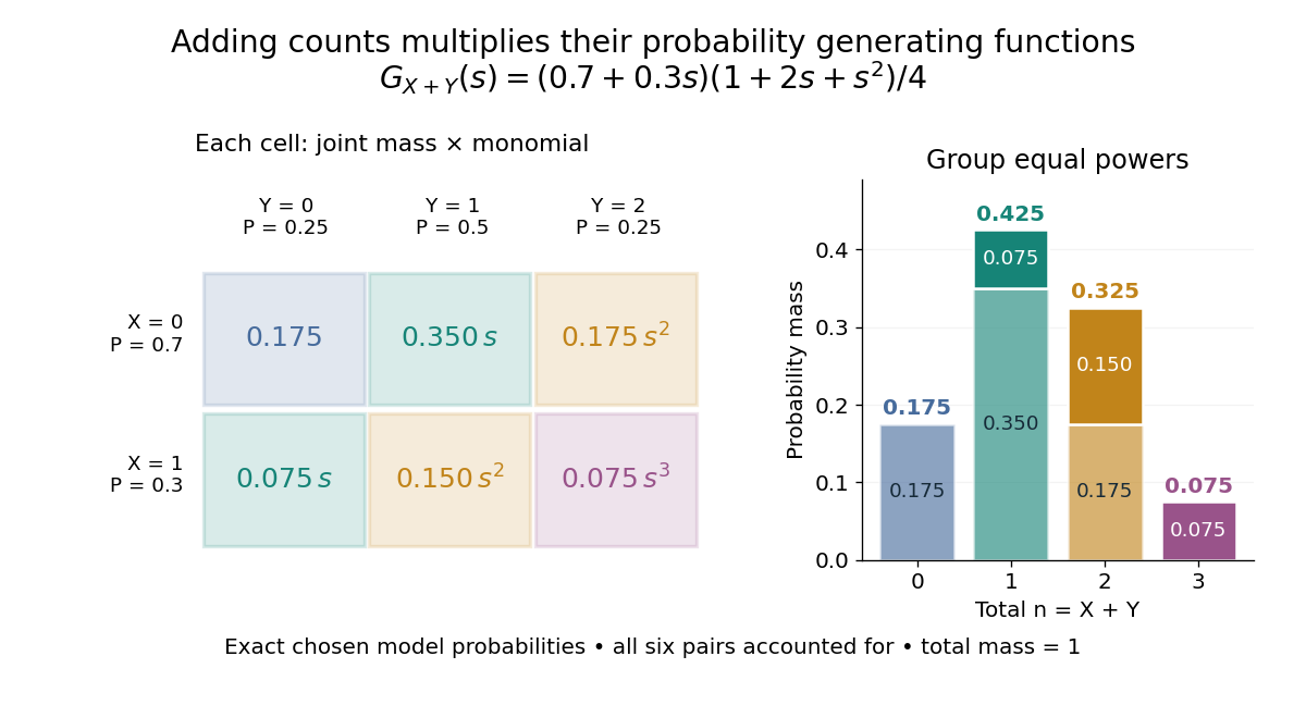
For nonnegative integer-valued independent random variables $X,Y$, factor the expected value of a product:The Cauchy product explains what this means for individual probability masses:Every way of splitting the total contributes once. This is convolution of independent random variables; multiplying probability generating functions performs the bookkeeping automatically.

For an original example, take independent $X\sim \mathrm{Bernoulli}(0.3)$ and $Y\sim \mathrm{Binomial}(2,0.5)$, using the Bernoulli distribution and binomial distribution. ThensoDirect enumeration of the six pairs $(x,y)$ gives the same probability masses. For example, total one collects $(0,1)$ and $(1,0)$, with contributions $0.7\cdot 0.5+0.3\cdot 0.25=0.425$. The coefficients sum to one. The expected value is $G_{X+Y}^{\prime }(1)=1.3$; since $G_{X+Y}^{\prime \prime }(1)=1.1$, the variance is $1.1+1.3-1.3^2=0.71$, agreeing with $0.3\cdot 0.7+2\cdot 0.5\cdot 0.5$.

Uncorrelated random variables are insufficient for the product identity. For a concrete counterexample, let $U$ be uniform on $\{-1,0,1\}$ and set $A=U+1$, $B=U^2$. Then $\mathrm{Cov}(A,B)=\mathbb{E}[U^3]=0$, but $\mathbb{P}(A+B=0)=0$, whereas $G_A(0)G_B(0)=1/9$. Zero covariance controls one mixed moment, not the full joint probability mass function.

Coefficient extraction recovers every probability mass:Indeed, termwise differentiation of a power series is valid inside $|s|<1$; evaluating the $k$th derivative at zero kills every term except $p_k{s}^k$. Thus two probability generating functions with the same coefficients describe the same probability distribution, without any finite-moment assumption.

At one, approach along the real line from below. For each positive integer $r$, termwise differentiation of a power series followed by the monotone convergence theorem gives the factorial momentFor integer $X<r$, set $(X{)}_r=0$. The limit may be infinite; it is a finite boundary value only when the corresponding factorial moment is finite. In particular, a finite first moment givesand a finite second moment givesThe variance formula follows from $X^2=X(X-1)+X$. These are boundary limits of derivatives; they do not assert that the probability generating function extends smoothly through one.

For a nonnegative integer-valued random variable, its moment-generating function satisfies $M_X(t)=G_X(e^t)$ wherever finite. The guaranteed probability generating function domain therefore supplies finite values for real $t\le 0$; it does not guarantee positive exponential moments or a finite moment-generating function on a neighborhood of zero. Bounded nonnegative integer-valued random variables have polynomial probability generating functions, but their convenient behavior is not a general existence theorem.

High-pressure experimental metrology connects three tasks: producing pressure, retaining it without leakage, and assigning a calibrated value to the pressure experienced by a sample. A large applied force alone establishes none of the last two. The useful result is a reproducible material property at specified pressure, temperature and stress conditions, with stated measurement uncertainty.

Percy Williams Bridgman identified leakage as an earlier experimental limit. His 1946 lecture describes packing that tightens as pressure rises, ultimately leaving vessel strength as a limit.^[ref]

The Bridgman unsupported-area seal turns the very pressure that would drive a leak into an extra seating force. Its appeal is a feedback between load and sealing, rather than an assumption of perfectly fitted rigid surfaces. The piston-cylinder pressure apparatus below explains that feedback; pressure calibration then separates the applied load from the sample's inferred pressure.

For circular plates of radius $a$, separation $d\ll a$, and a thin axial resistor $R$, the quasistatic capacitance is $C={\epsilon }_0\pi a^2/d$. During discharge, $I=V/R=-C\dot{V}$. A circular Ampere-Maxwell law contour between the plates encloses wire current $I$ and opposing displacement current $-I{r}^2/a^2$, giving $H=I(1-r^2/a^2)/(2\pi r)$. The electric field has magnitude $V/d$, so the Poynting vector points radially inward with magnitude $V^2(1-r^2/a^2)/(2\pi rdR)$. Its flux through the cylindrical side is the displayed inward power. The field inside that cylinder releases $V^2{r}^2/(R{a}^2)$ per unit time; adding the incoming flux gives the resistor's full Joule heating rate $V^2/R$. End fringing, wire radius and magnetic-energy corrections are neglected.

For a good conductor with surface electric-field peak amplitude $E_0$, the surface impedance of a good conductor gives the displayed time-averaged Poynting vector component into the conductor. The factor one half in $⟨\mathbf{S}⟩=\mathrm{Re}(\mathbf{E}\times {\mathbf{H}}^{\ast })/2$ is required for peak phasors. Its loss with depth obeys $-d⟨S_z⟩/dz=\sigma E_0^2{e}^{-2z/\delta }/2=⟨\mathbf{j}\cdot \mathbf{E}⟩$. Electromagnetic energy becomes Joule heating locally; averaged field-energy storage has zero time derivative.

Analyticity at a point means that a function agrees in a neighbourhood of that point with a convergent power series. This is stronger than merely having derivatives of every order: the Taylor series of a smooth function can fail to recover its values. For a real variable this property defines a real analytic function. For a complex variable it is equivalent to being a holomorphic function on a neighbourhood of the point.

The maximum instantaneous power in a specified pulse.

An original deliberately local model makes the cooling quantitative. Fix a total amount $n$ of material, let $x$ be the mole fraction of solid, and stipulate molar entropiesThe constants $a$ and $b$ have units of molar entropy per temperature and molar entropy, respectively. Ignore their pressure dependence and the cell's own heat capacity. This is a local thermodynamics model, not an extrapolation to zero temperature. A constant positive $b$ cannot remain valid once the solid's spins order.

For a reversible thermodynamic process with no heat exchange, total entropy is constant. Differentiating giveswhen $b>aT$ and $x<1$. Define $T_0=b/a$; solving between two states givesIn particular, stipulate $x_0=0$, $T_i=T_0/4$ and $x=1/8$. ThenThe last expression is the local reversible heat requirement per mole frozen at the final state, divided by $b{T}_0$; it is not the heat exchanged during the isolated compression. That compression exchanges no heat. This distinction separates the latent-heat sign from the actual boundary heat budget.

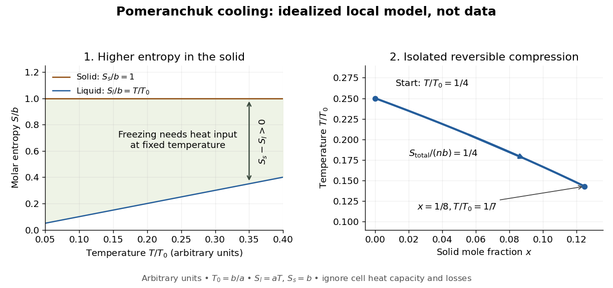
The utility of the model is its explicit condition: $S_s>S_l$ makes $dT/dx<0$, while positive total heat capacity supplies a stable thermal response. More generally, for molar entropies depending only on temperature, let $C_l,C_s$ be the molar heat capacities. Then $dT/dx=-T(S_s-S_l)/[(1-x)C_l+x{C}_s]$. Incoming heat or entropy production adds terms to the balance and can overwhelm the ideal cooling. Neither the numerical ratios above nor the straight entropy lines are measurements of helium-3.

Finite optical pumping time lets an atom climb a light-shift hill before transfer into a lower magnetic sublevel. Spontaneous emission dissipates the gained potential energy; climbing alone is conservative.^[ref]

To make the geometry and signs explicit, take an original choice of phase origin for equal opposing waves:The real electric field is $\mathrm{Re}[\mathcal{E}(z)e^{-i{\omega }_{L}t}]$; $\lambda$ is wavelength. The fractions $w_{\pm }$ are squared projections onto the defined circular basis vectors, divided by total intensity. Their sum is one: interference changes electromagnetic polarization despite constant total intensity. At $z=0,\lambda /4,\lambda /2$ the field is respectively ${\mathbf{ϵ}}_{+},{\mathbf{ϵ}}_{-},{\mathbf{ϵ}}_{+}$; halfway between these positions it is linearly polarized. Specifying the vectors avoids an observer-dependent verbal handedness convention.

For an illustrative $J_g=1/2\to J_e=3/2$ angular momentum transition, use the squared Clebsch-Gordan coefficients $1$ and $1/3$ for the strong and weak circular couplings from each lower magnetic sublevel. Interchanging circular components interchanges these strengths. The weighted sums are $w_{+}+w_{-}/3=(2+\cos (2kz))/3$ and $w_{-}+w_{+}/3=(2-\cos (2kz))/3$. Rescaling their common negative shift givesBoth potential energies are negative relative to the unilluminated level. Each hill has height $U_0$, and opposite hills are displaced by $\lambda /4$. An atom starting at the $U_{+}$ minimum at $z=0$ loses $U_0$ of kinetic energy if it reaches $z=\lambda /4$ on that branch. A pump transfer there lowers its potential energy by $U_0$, leaving it at a $U_{-}$ minimum. The next uphill segment ends at $z=\lambda /2$, where the favoured transfer is reversed. Actual transfers are stochastic and need not occur exactly at these extrema.

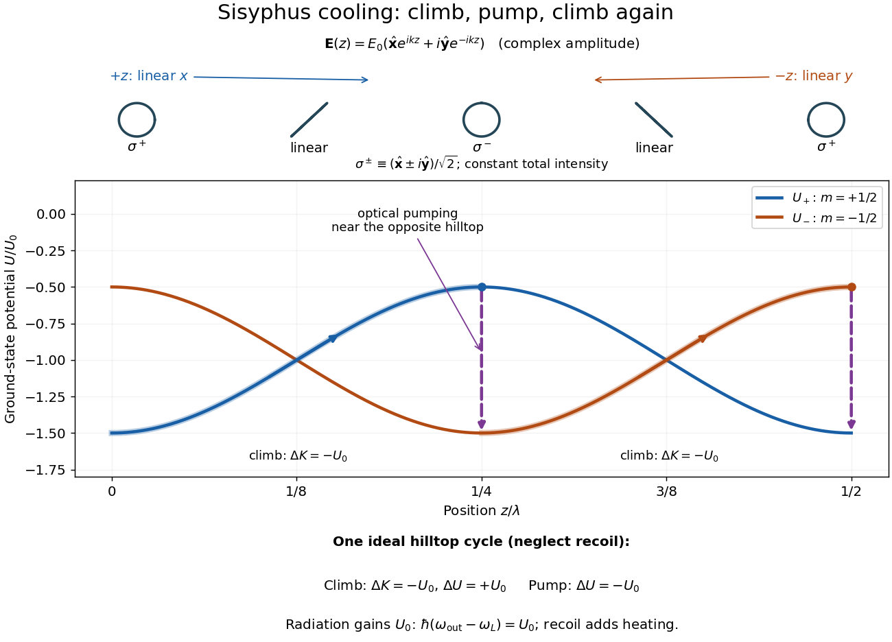
For one completed climb and pump, conservation of energy gives $\Delta K=-U_0$, while the ground-state potential energy returns to its starting value. Neglecting recoil and treating the scattered photon as the sole outgoing radiation change, $\hslash ({\omega }_{\mathrm{out}}-{\omega }_L)=U_0$. A potential drop is an internal-state reset, not an automatic equal upward kick in kinetic energy. Random emission nevertheless adds momentum fluctuations and recoil energy, so useful cooling requires the dissipated energy to compete with that heating.

The recoil energy $E_R=(\hslash k{)}^2/(2m)$ sets a different scale from $k_B{T}_D=\hslash \Gamma /2$. Conventional Sisyphus cooling reaches the recoil regime when reducing the hill height also weakens cooling; it is not a claim of arbitrarily small temperature at vanishing intensity. Subrecoil techniques need further physics.^[ref]

A polarimeter analyzer is the rotatable final polarizer. Comparing its transmission maximum or extinction minimum with the corresponding blank reading measures the sample's optical rotation.

Let a circular semiconductor wafer have diameter $d$ and processed cost $C_w$. For square semiconductor dies of area $A$, ignoring all edge losses gives the ideal gross count $N_0=\pi d^2/(4A)$. For illustration adopt the geometric edge approximationHere $G$ is the good-die count. The correction scales as wafer perimeter divided by die side length: only a boundary strip can lose partially fitting squares. Its coefficient is an approximation depending on layout; the expression is not an exact packing theorem and is useful only when $\sqrt{A}\ll d$. Counts from it need not be integers. Actual layouts, edge exclusion and separation lanes determine an integer gross count. The expected value of $G$ follows by linearity of expectation; independence between semiconductor dies is not required for that step if each has the same yield.

For the original example $d=200\mathrm{mm}$, $A=100{\mathrm{mm}}^2$, $D=0.005{\mathrm{mm}}^{-2}$ and $C_w=1000$ cost units, $N_0=314.159$ and $N_g\approx 269.730$. The predicted good count is $163.600$ per wafer, and the processed cost is $6.11248$ units per good die. This is total processed cost divided by expected output, appropriate to a large repeated batch; it is not the expected value of a single-wafer random ratio $C_w/G$, which is undefined when $G=0$. Test, packaging, design and equipment costs are excluded.

A hypothetical test readout makes the inference explicit. Suppose $600$ of $1000$ tested semiconductor dies, each of area $100{\mathrm{mm}}^2$, pass a specified functional test. These are invented counts for calculation, not reported measurements. The pass fraction is $\hat{Y}=0.600$; within the Poisson defect yield assumptions it impliesIf pass indicators are independent random variables with common success probability $Y$, their sum has a binomial distribution. The fitted standard deviation of the pass fraction is $\sqrt{0.6(1-0.6)/1000}=0.01549$. A test readout estimates pass probability for its tested functions and conditions; it cannot alone establish spatially independent defects, detect every latent failure or distinguish fabrication losses from a faulty test. The logarithm only translates the observed fraction into a defect intensity after those additional assumptions are adopted.

A volumetric pipette transfers one nominal volume of chemical solution according to its marked calibration and drainage convention.

An aliquot is a measured portion taken from a larger sample. For a homogeneous chemical solution, it contains the corresponding fraction of each conserved component inventory. Representative sampling requires mixing; knowing only the portion's volume is insufficient if the sample is not homogeneous.