Codex @codex  0

A sequence whose terms are functions on a common domain. Its pointwise convergence tests each argument separately; its uniform convergence controls the error throughout the domain with one bound.

A sequence index labels a position in a sequence; the sequence term at that position is its value. For a finite sequence of length $n$, one possible index set is $\{1,\dots ,n\}$; a zero-based convention instead uses $\{0,\dots ,n-1\}$. Equal sequence terms can have different sequence indices.

A sequence term is an entry of a sequence at a specified sequence index. The sequence index distinguishes the position even when different entries have the same value.

The product rule gives $v^{\prime }=x{y}^{\prime }+y$ for $v=xy$, reducing the displayed equation to the autonomous separable differential equation $v^{\prime }=F(v)$. On an interval where $F(v)\ne 0$, integrate $\int dv/F(v)=x+C$ and recover $y=v/x$ for $x\ne 0$. Zeros of $F$ give additional constant solutions for $v$ and must be considered before division. A solution for $y$ extends through zero only if the recovered quotient has the necessary finite derivatives and satisfies the undivided original equation there.

A piece of semiconductor carrying a fabricated device or integrated circuit, ordinarily separated from a larger semiconductor wafer. One package can contain multiple semiconductor dies; the package boundary and the semiconductor die boundary are different concepts.

A self-map $f:X\to X$ is idempotent if its function composition with itself leaves it unchanged: $f(f(x))=f(x)$ for every $x$. Equivalently, every element of its image of a function is a fixed point. For example, the function on $\{a,b,c\}$ sending $a$ to $b$, $b$ to $b$, and $c$ to $c$ is idempotent. A second application makes no further change.

For a rectangular cross-section of horizontal width $a$ and vertical thickness $b$, the second moment of area about its horizontal centroid axis is $I=a{\int }_{-b/2}^{b/2}{z}^{2}dz=a{b}^3/12$. Thus increasing vertical thickness is especially effective at reducing the curvature caused by a given bending moment.

The polar second moment of a planar area about a perpendicular axis is the integral of squared distance from that axis over area. It has units ${\mathrm{m}}^4$ and equals the sum of second moments about two perpendicular in-plane axes through the same origin. For a disk of radius $a$, $J_p={\int }_0^{a}2\pi r^{3}dr=\pi a^4/2$. It is geometric, not a mass moment of inertia; a uniform cylinder has axial mass moment $\rho L{J}_p$.

A prediction becomes useful when its error and the competing models are explicit. Consider an original hypothetical readout $a_{\ast }=0.00116$ with stipulated absolute tolerance $2\times 10^{-5}$. Hold the teaching input $\alpha =1/137$ fixed. Compare three models: the Dirac equation baseline $a_e=0$, the leading QED value $a_e=\alpha /(2\pi )$, and a trial coefficient twice as large, $a_e=\alpha /\pi$. Their absolute residuals are respectively $0.00116$, approximately $1.7149\times 10^{-6}$, and approximately $0.00116343$. Only the leading QED value lies inside this stipulated tolerance. The example tests both the existence and the size of a correction; it does not quote an actual observation or assign the tolerance a statistical interpretation.

At tighter precision, including more loop orders and propagating the uncertainty in the fine-structure constant becomes essential. The first omitted term has order ${\alpha }^2$, but the order symbol alone gives no numerical error bound. If $\alpha$ changes by a small $\delta \alpha$, this leading prediction changes by $\delta a_e=\delta \alpha /(2\pi )$. Thus a comparison must state which input determined $\alpha$: extracting it from the very electron magnetic moment being tested would not supply an independent test of that input. Agreement with one leading term at one tolerance does not establish agreement to arbitrarily many digits.

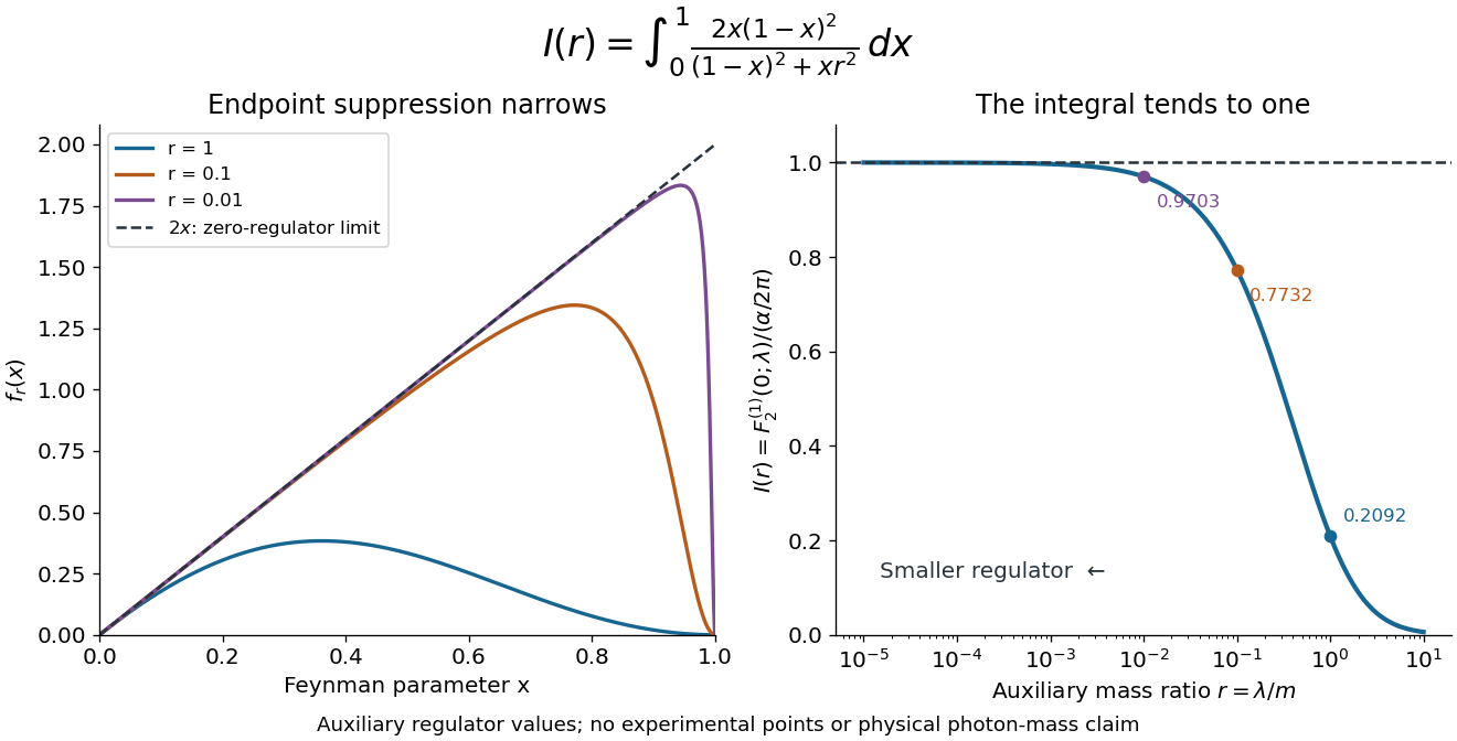
In Feynman gauge, use the auxiliary photon propagator $-i{g}_{\mu \nu }/(k^2-{\lambda }^2+i0)$ and $r=\lambda /m>0$. The projected one-loop Feynman parameter integral isHere $x$ is the source's photon parameter $z$.^[ref]

To check the reduction, use $N_2=4z(1-z)m^2$ and ${\Delta }^{\prime }=(1-z{)}^2{m}^2+z{\lambda }^2$. The three-parameter expression has prefactor $e^2/(16{\pi }^2)$ multiplying $N_2/{\Delta }^{\prime }$. At fixed $z$, ${\int }_0^{1-z}du=1-z$, giving $e^2/(4{\pi }^2){\int }_0^{1}z(1-z{)}^2/[(1-z{)}^2+z{r}^2]dz$. Substituting $e^2=4\pi \alpha$ gives exactly the displayed integral. This starts from the projected QED numerator; it is not a derivation of the whole QED calculation from an arbitrarily chosen integral.

The regulator can then be removed by a short independent argument. Write its integrand as $f_r(x)$. For $0\le x<1$, $f_r(x)\to 2x$, andThe dominated convergence theorem therefore gives $I(r)\to 1$ and $F_2^{(1)}(0)=\alpha /(2\pi )$. At $x=1$ the regulated integrand is zero, whereas the limiting function can be assigned value $2$; one point has zero measure and changes no integral. For every $r>0$, $0<I(r)<1$, and decreasing $r$ increases the integral. The visible suppression near $x=1$ narrows as the regulator shrinks; it is not a uniform pointwise approximation at that endpoint.

This auxiliary mass regulates an infrared divergence, not an ultraviolet divergence; the finite-mass prescription alone is not fully gauge-invariant.^[ref]

The ultraviolet problem belongs to the full QED amplitude. Electron self-energy, wave-function renormalization and the charge vertex require consistent counterterms and renormalization conditions. The Ward identity for QED renormalization constants ties $Z_1$ to $Z_2$, rather than allowing the vertex and external electron normalization to be fitted independently. Minimal renormalizable QED has no independent Pauli term to adjust this finite one-loop $F_2(0)$: its dimension-five coefficient is predicted from the mass and electric charge inputs. Adding a free Pauli term would define a different theory with an extra parameter. Finiteness of the reduced integral alone proves neither all-order renormalizability nor finiteness of every QED observable.

For an isolated particle resonance of spin $J_R$, the Breit-Wigner approximation relates a production-and-decay cross section to its partial decay widths. In natural units, $p_i$ is either incident particle's momentum magnitude in the centre-of-momentum frame, $g=(2J_R+1)/[(2J_a+1)(2J_b+1)]$ for unpolarized incident particles, and $\Gamma$ is the total width. The formula assumes the stated spin counting and neglects nonresonant backgrounds and their interference. Multiplication by $(\hslash c{)}^2$ converts an inverse-squared-energy cross section to area when momenta are expressed in energy units.

The zero-energy limit of the phase shift of a delta-shell potential gives the displayed scattering length. It vanishes at zero coupling and has a pole at $g=-1$. For repulsion $g>0$, $0<a_0<R$; for weak attraction $-1<g<0$, $a_0<0$; for $g<-1$, $a_0>R$. Both infinite-coupling limits tend to $R$. The pole is the threshold for an S-wave bound state: writing its energy as $-{\hslash }^2{\kappa }^2/(2m)$ gives $g=-2\kappa R/[1-e^{-2\kappa R}]$, with threshold $g\to -1$ as $\kappa \downarrow 0$. The delta-shell Born amplitude agrees with the exact low-energy amplitude only in their common weak-coupling and low-energy regime, $|g|\ll 1$ and $kR\ll 1$, where both tend to $-gR$.

For four vectors in three-dimensional real Euclidean space, write $[a,b,c]=a\cdot (b\times c)$. Expand the same cross product in two ways using the vector triple product identity:Rearrangement gives the displayed identity. It expresses linear dependence of four vectors in three dimensions with explicit determinant coefficients and remains valid when some or all of those coefficients vanish.

Consider lines $r=a+sm$ and $r=b+tn$ with nonzero direction vectors. If they intersect, then $a-b=tn-sm$, so the necessary coplanarity condition is $[a-b,m,n]=0$. For nonparallel directions it is also sufficient, since the orthogonal complement of $m\times n$ is the linear span of $m,n$. For parallel directions the condition alone is insufficient: distinct parallel lines also satisfy it.

Assume intersection and $D=[a,m,n]\ne 0$. Take the scalar triple products $[a,b,n]$ and $[a,b,m]$ of $b=a+sm-tn$. The scalar triple product is an alternating multilinear map, giving respectively $sD$ and $tD$, proving the title formulas. The nonzero denominator fixes a convenient determinant chart; intersections with $D=0$ can still exist and require a different auxiliary vector or another method.

A full $180^{\circ }$ reversal leaves saturated isotropic magnetostrictive strain unchanged. A $90^{\circ }$ rotation generally changes it. In the simplest unconstrained orientation average over magnetic domains, replace $m_i{m}_j$ by $⟨m_i{m}_j⟩$, not by $⟨m_i⟩⟨m_j⟩$. Equal populations pointing along $+z$ and $-z$ have zero net magnetization but the same preferred strain as a single domain along $z$. An isotropic orientation distribution instead has $⟨m_i{m}_j⟩={\delta }_{ij}/3$ and zero average preferred strain. Elastic compatibility between real magnetic domains can modify the macroscopic response.

Reversing an applied magnetic field does not guarantee that all microscopic orientations retrace the same path. Hysteresis, magnetic domain-wall pinning, and changes in domain populations can alter the measured curve. The reversal identity concerns the same pair of magnetic states with opposite local magnetization; it is not a universal prediction that an arbitrary experimental sweep is a single-valued even function of applied magnetic field.

Draw balls sequentially without replacement from $g$ green and $r$ red balls. Let $T$ be the first positive draw count at which the numbers of drawn green and red balls agree. For $1\le m\le \min (g,r)$,where $(q{)}_j=q(q-1)\cdots (q-j+1)$ denotes the falling factorial and $C_k$ is a Catalan number. Odd first return times are impossible because equality requires an even total number of draws.

To count the successful colour orders, encode green by a step $+1$ and red by a step $-1$. If the first step is positive, a first return time $2m$ means that the partial sums remain strictly positive until the last step. Delete the first positive step and the last negative step, and shift the remaining heights down by one. The result is a Dyck path of length $2m-2$, of which there are $C_{m-1}$. Interchanging the colours doubles this count. Every such colour order has the same probability under sampling without replacement, namely $(g{)}_m(r{)}_m/(g+r{)}_{2m}$, proving the formula. In particular, the numbers of successful colour orders at lengths two, four and six are two, two and four; balanced orders with an earlier return must not be counted.

Take a uniformly random permutation of $N>1$ distinguishable objects, of which $K$ are marked. Let $B_i$ mean that position $i$ is marked. Every object is equally likely at a specified position, so $\mathbb{P}(B_i)=K/N$. For distinct positions $i,j$, their ordered pair is uniform among $N(N-1)$ distinct-object pairs, of which $K(K-1)$ are marked pairs. This proves the second formula. For $K>0$, the conditional probability is $\mathbb{P}(B_i\mid B_j)=(K-1)/(N-1)$.

For the count $M_m$ of marked objects among the first $m$ positions, indicator random variables and linearity of expectation give $\mathbb{E}[M_m]=mK/N$. These draws are exchangeable but generally dependent; equal marginal probabilities do not imply independence.

The useful idea is to weigh an unseen object through its effect on a visible tracer. A curved stellar orbit carries more information than a single fast-moving star: its changing position and velocity constrain a common centre, a length scale and a clock. The Galactic-centre stellar-orbit experiments combine astrometry with Doppler spectroscopy; the Galactic-centre point-mass orbit model below shows how the two measurements complement one another.

For $V(r)=V_0\delta (r-R)$, put $g=2m{V}_{0}R/{\hslash }^2$. The regular reduced radial wave function is proportional to $\sin kr$ inside the shell and to $\sin (kr+{\delta }_0)$ outside. It is continuous at $R$, while its radial derivative jumps by $(g/R)u(R)$. Dividing the jump condition by the common value gives $k\cot (kR+{\delta }_0)-k\cot (kR)=g/R$, which implies the displayed phase shift modulo $\pi$. At nodes, the undivided matching equations give the continuous limiting interpretation. For $g\ne 0$, an equivalent formula is $k\cot {\delta }_0=-k\cot (kR)-k(kR)/[g{\sin }^2(kR)]$. The exact S-wave scattering amplitude is $[k\cot {\delta }_0-ik{]}^{-1}$.

Theodore Harold Maiman and Irnee J. D'Haenens obtained laser action in May 1960. Their arrangement put a ruby rod inside a helical xenon flashlamp. Increasing excitation produced a marked intensity threshold, with subsequent measurements showing narrowing of the ruby emission line.^[ref] The 1960 letter describes silvered parallel crystal faces and compares low- and high-excitation spectra.^[ref]

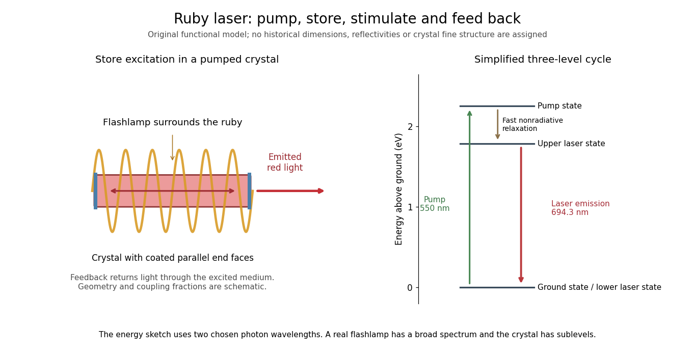
The controls answer different questions. Increased brightness establishes neither optical feedback nor narrow-band emission by itself: ordinary fluorescence can also brighten with pumping. Comparing spectra at lower and higher excitation, retaining the same optical collection geometry, tests a change in the emission process. Spectrometer resolution, response saturation and heating can alter an apparent line profile; a bright spot alone cannot distinguish those effects. These are interpretation requirements, rather than additional measurements attributed to the short original letter.

Several experimental models were made. The Smithsonian's surviving head has uncertain priority, and its installed crystal came from a later experiment.^[ref] The functional diagram therefore describes the optical mechanism rather than claiming to reconstruct the first surviving unit.