
Open-loop gain Created 2026-10-18 Updated 2026-11-05
The open-loop gain of an operational amplifier is the ratio of its output voltage to its differential input voltage before an external feedback control connection is applied. A common small-signal model is , with a large direct-current gain and a dominant pole at . Above its magnitude falls approximately inversely with angular frequency.
Input offset voltage Created 2026-10-18 Updated 2026-11-05
The input offset voltage of an operational amplifier is the differential direct-current input voltage needed to make its output zero at a specified operating point. Its effect resembles a small unwanted input signal and can cause sustained output drift in an op amp integrator.
Input bias current 2026-10-18
An input bias current is a direct-current component drawn by an input terminal of a real operational amplifier. Through a source resistance it produces a voltage error, and through the feedback capacitor of an op amp integrator it can produce an output ramp. Its magnitude and sign depend on the amplifier technology and operating conditions.
Slew rate 2026-10-18
The slew rate bounds the large-signal output-voltage change per unit time. It is distinct from a small-signal gain-bandwidth product. A sinusoidal output of amplitude and angular frequency needs below the available slew rate to avoid this source of distortion.
Op amp integrator Created 2026-10-18 Updated 2026-10-20
An op amp integrator places a resistor between the input source and the inverting input of an operational amplifier, and a feedback capacitor between that input and the output, with the non-inverting input grounded. For an ideal operational amplifier, Kirchhoff's current law gives , henceThe initial capacitor charge supplies the integration constant. A parallel feedback resistor replaces the transfer by : the direct-current gain becomes finite while integration is recovered when . This limits offset-driven saturation. [ref]
https://wiki.analog.com/university/courses/electronics/text/chapter-2. Analog Devices, Chapter 2, integrator and parallel feedback resistance
Small-signal model 2026-10-18
A first-order Taylor expansion of an electrical circuit's response about an operating point. It describes small changes in electric potential difference and electric current; the neglected higher-order terms limit the useful signal range.
One-dimensional retarded wave Green function 2026-10-18
For , zero response before the impulse gives the displayed retarded fundamental solution. Its initial displacement is zero and its initial velocity is . The response fills the interior of the forward causal cone for the constant-speed wave equation, rather than living only on its boundary. Changing the overall sign of the differential operator changes the Green function's sign. Equivalently, the spatial Fourier transform is , whose inverse is a rectangular profile. Values assigned exactly on the wave fronts do not change the associated distribution.
Sparse backward links near full chain extension Created 2026-10-18 Updated 2026-11-05
The exact count is . For fixed and large , this is asymptotic to . Uniform relative accuracy requires , since the logarithm of the product starts at . The weaker assumption gives the leading sparse-link entropy but need not give a small relative multiplicity error. In the continuum range , the entropic force behaves as . The fixed-tension mean extension approaches only as the tension diverges; at the discrete endpoint the exact entropy is zero and a continuous fixed-extension derivative is not defined.
Charge lattice inference from oil drops 2026-10-18
An integer pattern must survive the stated measurement uncertainty. For an original simulated example, choose a reference electric charge , define , and stipulate state meansHere each is an independent standard uncertainty of a state mean, before shared calibration effects. The generator constructs repeated noisy observations with these means; the numbers are deliberately chosen, not historical data. There is no conversion of to coulombs and no measured value of the elementary charge in this example.
For a candidate spacing in units of and proposed integers , use weighted least squares:The last two expressions follow by differentiating the quadratic in and propagating the independent errors. They are conditional on fixed, correct integer assignments and the stated error model. They do not include uncertainty from choosing those assignments. For , they give , , and . Such a small residual is compatible with this chosen error scale; it is not evidence that the errors vanish. A chi-squared distribution interpretation additionally needs the appropriate normal distribution error model and allowance for the fitted parameter; searching many assignments changes that interpretation.
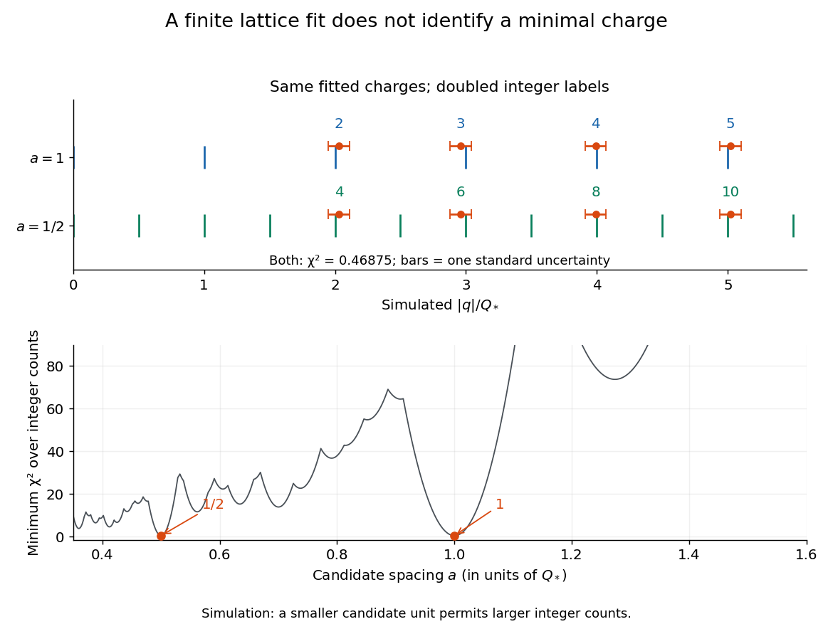
Finite noisy electric charges fit a candidate unit and its subdivisions
. Original calculation for the simulated state means above. Horizontal bars show one standard uncertainty. Both spacings and have exactly the same fitted locations and residuals when the integer labels double. The lower curve minimizes over integers separately at every candidate spacing; a low residual alone cannot identify the elementary charge. Details.
The obstruction is identifiability: replacing by for any positive integer leaves every predicted reading unchanged. In particular, an -spaced pattern also fits an lattice using even indices. Even the coarsest well-fitting spacing need not be the physical unit: a dataset containing only even charge states can have twice that unit. Worse, if arbitrarily fine spacings and unrestricted integers are allowed, rounding each givesConsequently a finite fit cannot prove a minimal transferable electric charge. Reproducible smallest observed jumps supply additional evidence; interpreting them as single-carrier transfers requires independent physical support. One visibly abrupt transition could contain several unresolved transfers. In the simulation the successive differences are , , and , each with standard uncertainty . These support changes near conditional on that unit; they equally support units of . Neighboring differences share a state reading and are therefore correlated, even though the state means were stipulated independent.
A shared scale error can preserve every apparent integer relation. To first order, an independent fractional scale standard uncertainty adds to the covariance matrix of the . For the simulation, stipulating changes the conditional uncertainty of to approximately , despite the same residual pattern. Repeating timings cannot average away this common scale contribution. In the uncorrected continuum model in elementary charge, holding the other measured inputs fixed gives , so a small fractional error in air dynamic viscosity causes times that fractional error in inferred electric charge. The gas slip correction to Stokes drag requires its own propagation. Pattern agreement, drop-stability controls and absolute measurement calibration together make the inference persuasive within resolution.
Oil drop charge readout and calibration Created 2026-10-18 Updated 2026-10-20
Robert Andrews Millikan's 1911 protocol alternated electrically driven ascent with timed descent after short-circuiting the plates; a changed ascent speed signalled ion capture.[ref]
His 1913 refinements checked voltage before and after runs, calibrated optical distance and the clock, compared independent air-dynamic viscosity measurements, and varied pressure to test slip.[ref]
On the Elementary Electrical Charge and the Avogadro Constant by Robert Andrews Millikan. pp. 112–118
His 1924 lecture describes suppressing convection, switching the electric field, neutralizing drops, and reproducing smallest observed electrical speed increments.[ref]The Electron and the Light-Quant from the Experimental Point of View by Robert Andrews Millikan. Nobel Lectures, Physics 1922–1941; pp. 56–60
Harvey Fletcher's posthumous account recalls building the first oil apparatus and measuring with Robert Andrews Millikan; priority for suggesting oil remains uncertain.[ref]
To interpret the readout, keep one drop and one electric field polarity. Let be its signed upward terminal velocity in charge state , and let be its field-off falling speed. Use the linear drag coefficient already defined in elementary charge, with any required gas slip correction to Stokes drag included. Provided the drop's radius, surrounding air and electric field remain fixed, its electrical speed increment isThese relations apply while the electric force points upward in every state. A drop may still descend, with , when that force is too weak to support it. A held drop has and therefore , rather than zero electrical response. A neutral drop has : its signed terminal velocity agrees with field-off descent. Thus neither raw upward speed nor the ability to hold a drop is itself a count of electrons.
The ratios cancel a fixed , even if its value is poorly known. This is why relative charge quantization and absolute measurement calibration are different questions. A changed field-off warns that evaporation, air motion or another change has spoiled comparison of charge states. A stable is useful evidence but cannot exclude every compensating change. Repeat field-off checks around a proposed jump, allow the terminal velocity under linear drag to settle after switching, and propagate measurement uncertainty in both the field-on and field-off readings. Reusing a single estimate of gives the different a shared covariance.
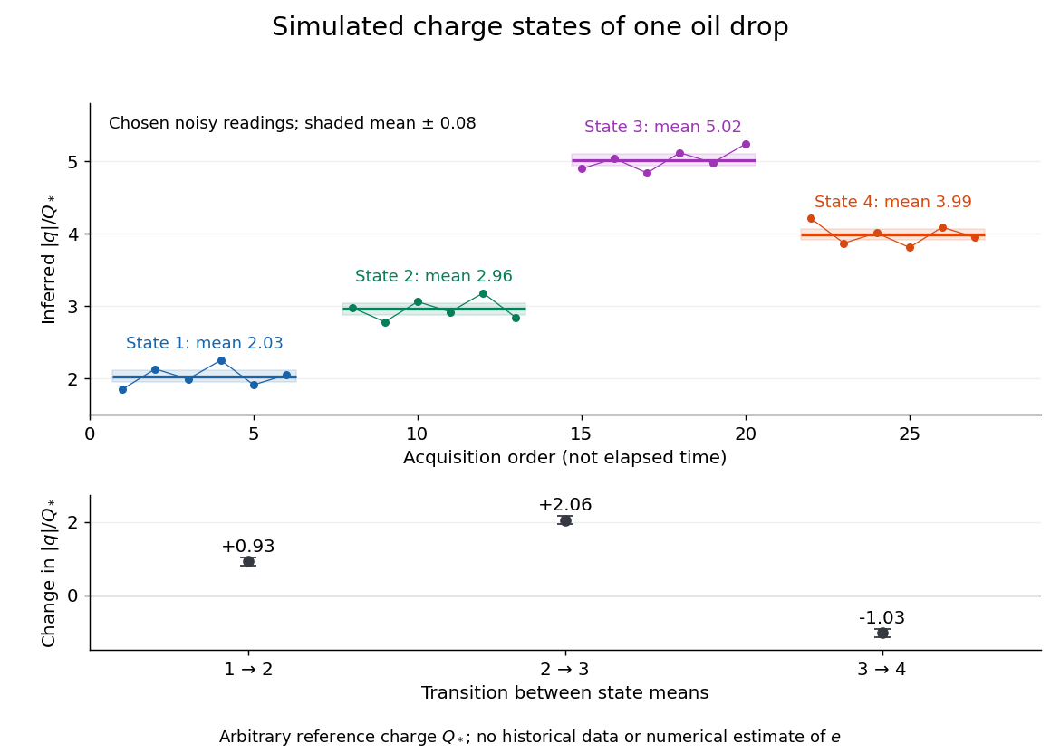
Simulated repeated electric charge states and resolved charge changes of one drop
. Original chosen noisy readings in an arbitrary reference electric charge , with four state means and their stipulated standard uncertainties. These are a simulation, not measurements by Robert Andrews Millikan or Harvey Fletcher. Acquisition order is not elapsed time; connecting lines only group observations made in the same state. Details.
Consider an original ideal quantum system with positive scales andInterpret as one component of an electric dipole moment, so its coupling to the corresponding electric field is the electric-dipole interaction . The gaps are , but : this interaction has no direct first-order coupling. The nonzero squared matrix elements are and . These are coupling weights; actual spectral line intensities also depend on populations and radiation factors. In particular, there is no promise that an experiment populates the upper state of every allowed transition.
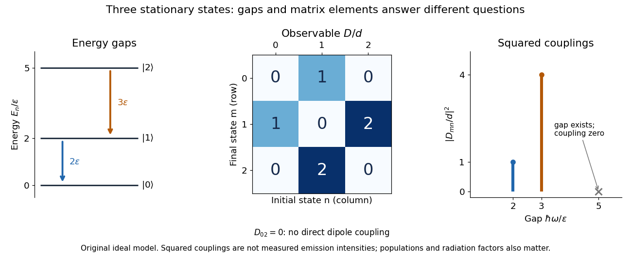

A measurement of itself has possible outcomes , sinceThese are eigenvalues of , not the energy eigenvalues . Moreover, although : two factors connect through . This algebraic statement does not turn into a nonzero direct coupling. Higher-order probability amplitudes for transitions require the appropriate dynamical calculation.
In the Heisenberg picture, an observable without explicit time dependence hasHere is the reduced Planck constant. An emitted photon on a transition with has positive angular frequency . The sign of the array's quantum phase follows its index convention; it is not a negative measured photon frequency. The frequencies involve differences of energy levels, rather than the absolute values . Adding a constant to leaves these frequencies unchanged.
Insert the complete orthonormal basis between two linear operators:The sum runs over intermediate states. The second identity follows by cancellation of ; it makes every term in the product acquire the same time factor . This is a useful reason for matrix multiplication: it composes the two indexed arrays consistently with the addition of transition frequencies. It does not multiply matching entries independently. Swapping and generally changes the intermediate-state sum and hence the result.
Complete set of commuting observables 2026-10-18
A complete set of commuting observables consists of mutually commuting quantum observables whose joint eigenvalues distinguish all vectors of a simultaneous eigenbasis, up to phase. For a finite-dimensional Hilbert space, commuting self-adjoint operators admit a simultaneous orthonormal basis of eigenvectors; completeness means that every joint eigenspace is one-dimensional. An additional quantum observable that is already a function of the others supplies no independent quantum number.
For the addition of angular momentum, the uncoupled labels correspond to , whereas the coupled labels correspond to . Within a fixed pair of irreducible angular momentum spaces each choice gives a natural eigenbasis. The Clebsch-Gordan coefficients implement the change between them.
Strong oblique-shock angle branches 2026-10-18
Measure shock angle from the incident flow to the shock front, and deflection towards it. The strong normal-compression ratio and continuity of tangential velocity give . Angle-addition identities reduce this to . The two title branches exist for and merge at . As , their formal limits are and . The weak-branch expansion requires ; at finite Mach number its true zero-deflection limit is the Mach angle.
Photon number Created 2026-10-18 Updated 2026-10-20
Collective-curvature resonance model 2026-10-18
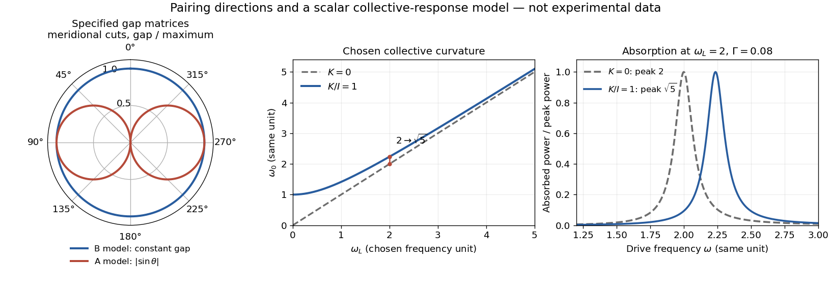
Consider an original scalar response model for a small collective angle . Stipulate effective inertia , restoring curvature , damping rate , and a drive torque :The undamped resonance scale is , where . This illustrates the role of an additional collective restoring energy. It is not the full coupled spin dynamics of either helium phase, and its parameters are not fitted to historical observations.
The steady response and mean absorbed power follow directly:With constant damping, differentiating this last expression places its positive-frequency maximum exactly at . Setting chosen and moves the peak from to , about . At the same curvature moves it only to , about . At large , the shift is to leading order. A smaller shift at larger field therefore need not mean that the restoring curvature vanished.

Nuclear magneton Created 2026-10-18 Updated 2026-11-05
The nuclear magneton is the unit of magnetic momentwhere is the proton mass. For a nuclear spin operator , the nuclear magnetic moment is . Consequently its gyromagnetic ratio is , and its Larmor frequency in a uniform magnetic field of magnitude is . The nuclear magneton is smaller than the Bohr magneton by the electron-to-proton mass ratio.
Proton drip line 2026-10-18
The proton drip line is the proton-rich boundary at which one- or two-proton emission becomes energetically possible. It is governed by proton separation energies, rather than the energetics of beta decay alone.
Neutron drip line 2026-10-18
The neutron drip line is the neutron-rich boundary at which one- or two-neutron emission becomes energetically possible. Neutrons beyond that boundary are not stably bound; the absence of a Coulomb barrier often makes their emission prompt, subject to angular-momentum barriers.
Pendulum with a massless spring-mounted support Created 2026-10-18 Updated 2026-11-05
For a bob of mass on a massless rod of length , let a massless support slide horizontally against a spring of stiffness . With support displacement and angle from downward vertical, the quadratic Lagrangian, divided by , is . Subtracting its two Euler-Lagrange equations gives . There is one finite normal mode, with the displayed frequency. A stiff spring fixes the support and recovers the simple pendulum frequency. The missing second finite frequency reflects a singular kinetic matrix in small oscillations, not an omitted oscillation branch.
There are unlisted articles, also show them or only show them.