
In 2006, Yilong Han and colleagues dispersed plastic ellipsoids in water inside a thin glass cell, using a very dilute suspension to limit particle interactions. A camera on an optical microscope recorded 30 frames per second. Image analysis extracted centre positions and long-axis angles, with reported angular resolution about . Their shape supplied the observable axis. Reflected interference colours calibrated cell thickness; nearly constant particle interference colour checked vertical wandering. One tracked particle had dimensions in an gap. Angular displacement variance grew linearly with lag; displacement resolved along the particle's axes and in the laboratory showed how turning washes out translational anisotropy. These are observations of confined particles: walls alter drag, and slight out-of-plane tumbling affected positional resolution. They do not establish the bulk sphere formula. The paper's Figure 1A–B shows simulations; Figure 1F shows a measured trajectory.[ref]
Brownian Motion of an Ellipsoid by Yilong Han and others. Han et al., Brownian Motion of an Ellipsoid, Science 314 (2006), pp. 626–628; Figures 1D–F and 2A–B: apparatus, angular readout, dilution and height checks, angular variance and translational crossover
For interpreting such images, the director distinction is essential: identical ends give an angle modulo . A continuously unwrapped trace can follow small successive turns, but it does not make the ends physically distinguishable. The invariant planar axis autocorrelation is , and its decay determines through . Separately measuring position and rigid body orientation is what makes the connection between translational anisotropy and loss of angular memory experimentally accessible.
Rotational diffusion of a sphere 2026-10-18
For a sphere of radius in an otherwise stationary, unbounded Newtonian fluid with dynamic viscosity , impose the no-slip boundary condition and the slow-flow assumptions of Stokes flow. The resisting torque on a rotating sphere in Stokes flow is , where is its angular velocity and . Thermal rotational diffusion at absolute temperature then givesHere is the Boltzmann constant; the translational expression is the Stokes–Einstein relation. The ratio has units of inverse length squared, so comparing the numerical values of and without their units is meaningless. At fixed temperature and dynamic viscosity, decreasing radius tenfold increases a thousandfold but only tenfold. This strong size dependence explains why small particles can lose directional memory extremely quickly.
Choose and as illustrative model inputs. Using gives and the following predictions:These are bulk three-dimensional sphere calculations, explicitly not a fit to the confined ellipsoid experiment below. Walls, nonspherical shape and departure from the no-slip boundary condition can change rotational resistance. A visible surface mark is still necessary to read the sphere's turning in an image, even when its rotational diffusion coefficient is well defined physically.
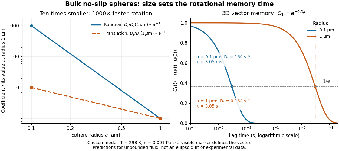

For isotropic turning in three dimensions, the tip of a marked unit vector wanders over the unit sphere. Its probability density function obeys the orientational Fokker-Planck equationHere is the Laplace-Beltrami operator on the unit sphere. The factor two follows from the sphere surface derivative identities: , so each mean vector component decays at rate . This is a different orientation space from the circle of planar rotational diffusion, whose corresponding rate is . For the same illustrative and , this three-dimensional autocorrelation is .
One unit vector records a pointing direction, not every aspect of a rigid body's rigid body orientation: rotation about that vector remains unspecified. Also, requires an identifiable arrow. An unmarked ellipsoid's long axis alone does not supply one, and projecting a three-dimensional trajectory onto a camera plane does not automatically produce the planar model.
Planar rotational diffusion 2026-10-18
For free planar turning with constant , no imposed torque and negligible inertia, model an unwrapped angle by the stochastic differential equationHere is standard one-dimensional Brownian motion, with increment variance , and brackets denote expected values over repeated realizations. The angular variance is conventionally reported in . “Unwrapped” means recording accumulated turns continuously, rather than resetting the angle at each revolution. Directly subtracting wrapped camera angles creates artificial jumps; for an unmarked ellipsoid the wrapping period is , and resolving successive turns additionally requires sufficiently frequent images.
For a planar arrow , the orientational autocorrelation isFor an unoriented planar axis, use an autocorrelation unchanged by replacing either endpoint angle by that angle plus :The same thus gives arrow and axis correlation times and , respectively, where a correlation time here is the lag at which the relevant curve reaches . A short explanation is enough: has a Gaussian distribution of variance , so its characteristic function gives . The integer selects what the observable can distinguish; it does not change the underlying angular spreading.
For an original numerical example, choose . After , the angular variance is and its root mean square displacement is , although the mean displacement is zero. The planar arrow autocorrelation is , while the planar axis autocorrelation is . Calling both “the orientation correlation” without specifying the observable would hide a factor of four in decay rate.
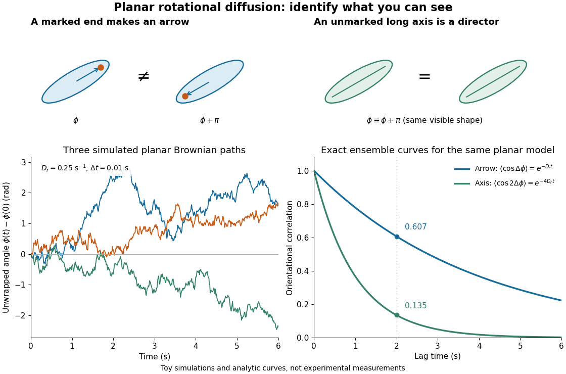
Planar rotational diffusion: arrows, unoriented axes and loss of angular memory
. Original schematics, three simulated Brownian motion angle paths and exact ensemble autocorrelation curves for the chosen . The paths use independent Gaussian distribution increments of variance with . The curves are model predictions, not fits to these three paths or experimental measurements. Both curves concern planar turning; neither is the three-dimensional unit-vector law. Details.
Equatorial Coriolis deflection in free fall 2026-10-18
A body released from rest relative to Earth at the equator has unperturbed downward velocity . The Coriolis acceleration in local Earth coordinates gives eastward acceleration . Integration gives and impact time , proving the title formula. This is first order in Earth's rotation, neglecting air resistance and the height dependence of the effective local gravitational acceleration. For a short fall at latitude , its leading eastward term is multiplied by .
Complex root 2026-10-18
A root of a polynomial lying in the complex numbers. It may be real: a nonreal complex root has nonzero imaginary part.
For rolling without slipping inside a stationary circular cylinder, take the inner body's axial moment of inertia to be . Its center of mass follows a circle of radius , and the reduced Lagrangian is . The Euler-Lagrange equation gives . Linearizing near the lowest position yields the displayed small oscillation frequency. A uniform solid cylinder has . This reduction requires sustained contact and enough static friction to prevent slipping.
Work by Robert E. Kass Created 2026-10-18 Updated 2026-10-25
In units , a receiver on the hyperbolic motion worldline , has retarded null coordinate . A right-moving light ray emitted at has , so it meets the receiver only if . The photon wave covector is proportional to , and contraction with the receiver's four-velocity gives its measured frequency as . The intersection condition gives the second displayed equality. Emission at lies on the Rindler horizon and never reaches the receiver at finite proper time; is the supremum of receivable emission times, not an attained latest time.
Light reception by a uniformly accelerated observer Created 2026-10-18 Updated 2026-10-20
Let an observer start at rest at , and accelerate towards increasing with constant proper acceleration . A signal emitted simultaneously from travels along . The observer follows hyperbolic motion, and . Their intersection obeysA finite future reception exists only for . At equality the ray lies on the limiting null horizon and never reaches the observer; for larger separation it remains outside the observer's receivable past. The proper reception time tends to as . The simultaneous emission and initial-rest conditions are essential; changing either changes the timing problem.
Geometric partition bounds for a power-law improper integral Created 2026-10-18 Updated 2026-10-25
On the geometric progression , with , the interval widths are . The left-endpoint Riemann sum for the decreasing integrand is the geometric seriesThe right-endpoint sum is . Integral comparison on each interval gives . Both bounds tend to as , proving the improper integral by the squeeze theorem. Although the largest interval width is unbounded on the infinite domain, these explicit upper and lower bounds justify the limit without incorrectly applying a finite-interval mesh argument to the entire half-line.
Retarded Fourier pole prescription 2026-10-18
For inverse time Fourier transform , a causal stable oscillator has its poles below the real frequency axis. Undamped real poles are therefore displaced by the prescription in its frequency polynomial. For , closing the contour below encloses poles with clockwise orientation; for , closing above gives zero. Changing the transform's sign reverses the corresponding prescription. For a positive oscillator operator , the inverse is and its time response is .
Exact polynomial steps for a delay equation 2026-10-18
Use the Malthusian delay differential equation with time measured in units of its constant delay:Here is a real constant. On the first interval , hence . On the next interval the delayed input is , already known, so the method of steps for a delay differential equation givesEach polynomial integrates the preceding interval's delayed polynomial, and its integration constant ensures continuity. At , the step endpoints are , , and . At , the value is , but its derivative is the earlier value . This is the geometric distinction from the ordinary differential equation , whose derivative would equal its current value.
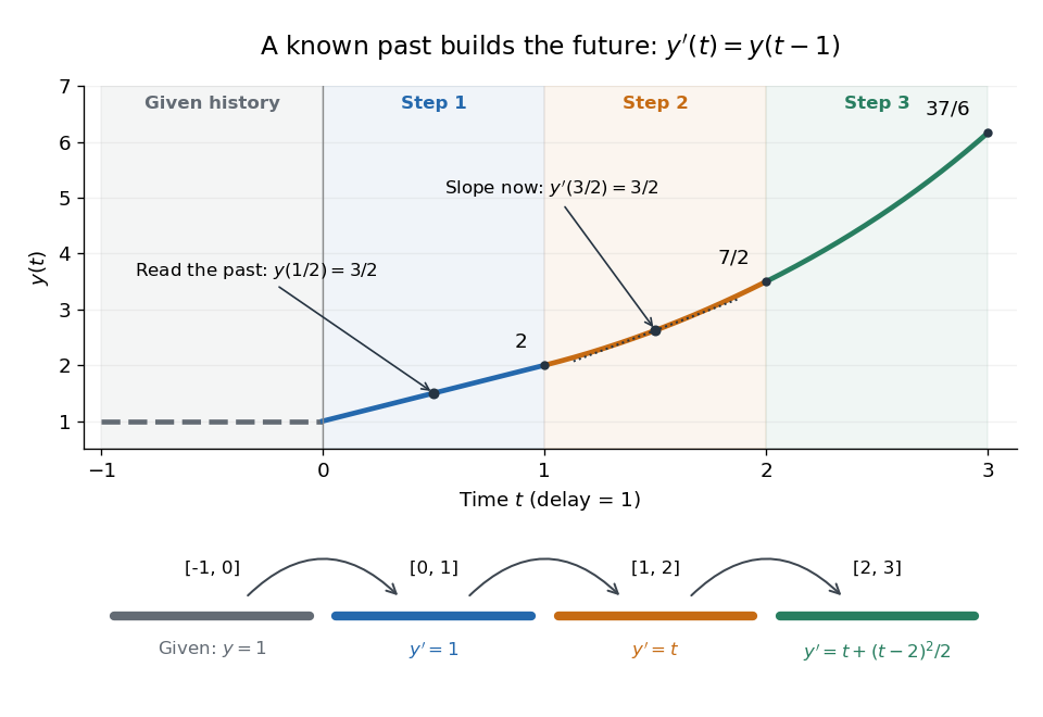
A prescribed past becomes successive exact polynomial steps
. The history function of a delay differential equation is and . Each colored interval supplies the delayed input for the next one; the lower panel gives that next interval's derivative. The marked tangent line at has slope . All curves are evaluated from exact polynomials. Details.
More generally, for any integer ,At an integer join the newly introduced term vanishes. Inside a step, differentiation lowers each power by one and gives exactly times the preceding step evaluated at . Together with , this verifies the formula by mathematical induction; it is an exact construction, not a truncated power series.
The history and the new equation need not prescribe matching derivatives at the starting time; their mismatch can reappear later in higher derivatives.[ref]
Delay-differential equations by Skip Thompson. Skip Thompson, Delay-differential equations, Derivative Discontinuities: initial incompatibility and its propagation
In this example, and . For , is continuous at but jumps there by ; at , the first jump is in , of size . The solution of a differential equation is therefore continuously differentiable for positive time, although it need not have continuous derivatives of every order at step boundaries.A history function of a delay differential equation supplies the past interval needed to start a retarded delay differential equation. A single initial condition generally leaves earlier delayed values unspecified.[ref]
Delay-differential equations by Skip Thompson. Skip Thompson, Delay-differential equations, Initial History Function: prescribing the solution before the starting time
For a continuous function history, the natural state at time is the entire segmentIt belongs to the function space , an infinite-dimensional vector space: the functions are linearly independent. Shifting forward retains the part of the past that the equation can still read. Thus even one scalar unknown can require a state in an infinite-dimensional vector space.
The insufficiency of one value is visible without any approximation. Consider with the two history functions of a delay differential equationBoth give , yet on the first step the respective derivatives are and . Direct integration givesIn particular while . On the next step,At they are and , a gap of . These different futures reflect different prescribed histories; each fully specified problem has a unique solution of a differential equation. More strongly, for with , observing the entire first-step derivative recovers every history value through for , using the right derivative at . The future can depend on the whole function, rather than a finite list of its samples.
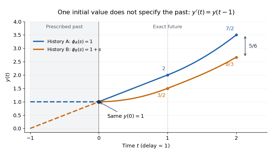
Equal initial values and different histories give different futures
. Two exact solutions of a differential equation for . Dashed curves are the prescribed history functions of a delay differential equation; solid curves are their exact continuations. Both pass through . The endpoint values and come from the displayed polynomials, with no numerical time stepping. Details.
Raman sideband cooling experiment of 1995 2026-10-18
In 1995, Christopher Monroe and collaborators cooled one ion in a ring/endcap Paul trap. They used Doppler cooling and optical pumping into . Red-sideband Raman transitions transferred population to , followed by dissipative recycling. Repeating across three directions yielded a reported three-dimensional ground state population of about .[ref]
Resolved-Sideband Raman Cooling of a Bound Atom to the 3D Zero-Point Energy by Christopher Monroe and others. Monroe and others, Resolved-Sideband Raman Cooling of a Bound Atom to the 3D Zero-Point Energy, 1995, pp. 4011–4013, Fig. 1 and Table I
A variable-frequency Raman transition probe, an exchange pulse and a cycling detection beam converted state populations into fluorescence collected through optics onto a position-sensitive photomultiplier. Red/blue asymmetry inferred motional occupation; varying probe duration tested the thermal assumption. Off-resonant processes and independently observed heating limited cooling.[ref]
Resolved-Sideband Raman Cooling of a Bound Atom to the 3D Zero-Point Energy by Christopher Monroe and others. pp. 4012–4014, Fig. 2, Table I and final heating discussion
From renormalizability to electroweak predictions Created 2026-10-18 Updated 2026-10-20
The 1999 recognition of Gerard 't Hooft and Martinus J. G. Veltman concerned the theoretical quantum structure of the electroweak interaction.[ref] Renormalizability makes repeated radiative corrections predictive from a fixed set of inputs. It does not imply that the perturbation series converges, nor that renormalization alone chooses the correct particle content or excludes all physics beyond the Standard Model.
The Gargamelle collaboration prepared an experimental test by exposing its heavy-liquid bubble chamber to neutrino and antineutrino beams at CERN. The readout selected events producing hadrons without an identified muon or electron, compared with events containing a charged lepton. Its 1974 report assessed alternative origins from neutrons and long-lived neutral kaons, finding them insufficient to explain the sample. That supported neutral currents; it did not isolate a radiative correction or demonstrate renormalizability.[ref]
The distinction matters when using the tree-level electroweak gauge-boson masses:Beyond tree level, self-energies, interaction vertices and counterterms alter how chosen input observables predict another observable. The Weinberg angle then needs a specified renormalization scheme; inserting its value from one convention into a formula from another can create an apparent discrepancy. A meaningful higher-order test must state both its independent experimental inputs and the calculated loop order.
The following scalar toy isolates one step in renormalization: removing a local divergence while retaining a finite dependence on a physical mass. For and a sharp cutoff regularization in Euclidean space with momentum bound , define the dimensionless Feynman integralThis is a zero-external-momentum scalar bubble integral stripped of coupling and combinatorial factors. Using the three-sphere area and reduces the integral toThe antiderivative follows by writing . At large the divergent part is , with the logarithm's dimensionful argument understood only within the displayed ratios. It has no external-momentum dependence. In a four-scalar-field vertex this structure can therefore be removed by a local operator proportional to , rather than a momentum-dependent nonlocal interaction.
Choose the fixed reference mass and subtract . If the loop contribution to a chosen four-point vertex coefficient is , choose the additive counterterm in that same coefficient as , where includes its stated diagram factors. This defines a finite subtraction prescription:The renormalization condition for this toy loop contribution is . The reference mass stays fixed when is varied; finite dependence on survives. A different finite subtraction changes the renormalization scheme, and the defined renormalized coupling must change consistently.
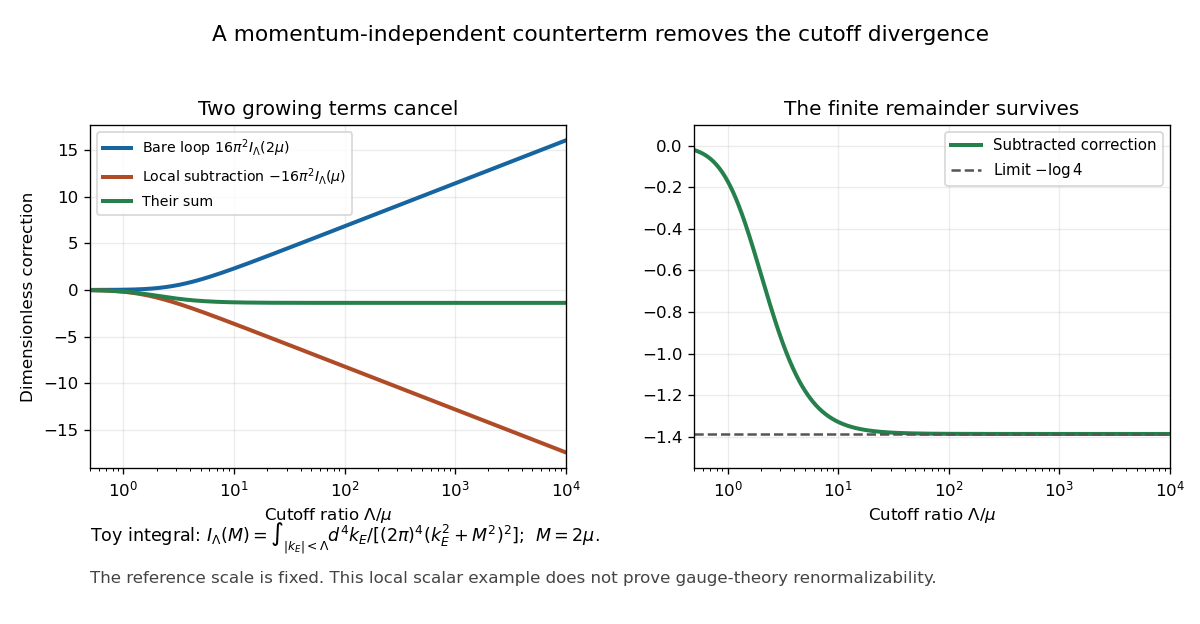

For , the limiting result is . At , the exact regulated difference is about ; at , it is about . Expanding the exact expression gives the leading residual in . This explicitly separates finite-cutoff error from the chosen finite renormalization condition.
A sharp cutoff regularization is convenient for this scalar demonstration, but shifts of a divergent loop momentum can change its integration domain. A gauge theory calculation cannot assume that it preserves the Ward identities. The toy contains no interacting gauge bosons, ghost loops or overlapping ultraviolet subdivergences, so its successful subtraction does not prove Non-Abelian gauge theory renormalizability.
Massive-vector propagators at large momentum 2026-10-18
Consider one massive gauge field with after Higgs mechanism. For this comparison perform a Wick rotation and take a real nonzero momentum in Euclidean space . The transverse and longitudinal orthogonal projectors areHere “longitudinal” means parallel to the off-shell four-momentum, not the physical longitudinal polarization of an on-shell massive gauge boson. The R-xi gauge quadratic vector operator and its inverse areMultiplication verifies , since and . The unitary gauge vector operator lacks the gauge fixing derivative term in the longitudinal sector, givingThus every eigenvalue of falls as at fixed finite positive , whereas has the constant longitudinal eigenvalue . Unitary gauge consequently obscures ordinary power counting; this is not a failure of the physical theory.
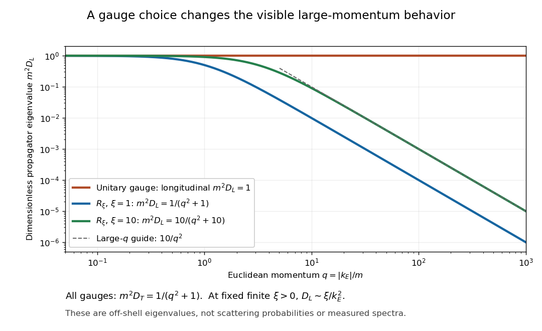

For a worked comparison choose . The dimensionless longitudinal eigenvalue is in unitary gauge, at , and at . Its crossover is : taking first gives a constant, whereas taking first gives zero. The two limits do not commute. Contracting the propagator between conserved external conserved currents projects away , but one cannot impose that simplification separately on every internal line of an interacting Non-Abelian gauge theory.
Polynomial remainder theorem 2026-10-18
Dividing a polynomial by leaves the constant polynomial remainder . Polynomial division makes the polynomial remainder constant because its polynomial degree must be below one; polynomial evaluation at identifies that constant. In particular, it is zero exactly when is a root of a polynomial of , which is the factor theorem.[ref]
Fields and Galois Theory by James S. Milne. Fields and Galois Theory, version 5.10, Chapter 1, p. 10, §1.7: division by X−a and evaluation of the constant remainder
In the worked example, division by leaves and division by leaves . Division by their product leaves , a polynomial remainder that stores both values at once. The argument also holds over a commutative ring for in that ring, because is a monic polynomial.
Charged relativistic dust Created 2026-10-18 Updated 2026-10-20
For identical particles of rest mass and electric charge , the four-current is . The matter stress-energy tensor obeys , with the opposite force density in the electromagnetic stress-energy tensor. Antisymmetry of the electromagnetic field tensor makes its contraction with two four-velocities vanish, so mass continuity still holds. Removing that term leaves the displayed covariant Lorentz force law. The matter tensor alone is not divergence-free when an electromagnetic force acts.
There are unlisted articles, also show them or only show them.