
Strong induction for factorization existence 2026-10-18
Every integer has a prime factorization. The induction base case is prime. For a larger integer, either it is prime or it is , with . The induction hypothesis supplies prime factorizations of both smaller integer divisors; multiplying them gives one for . This proves existence, while uniqueness requires the additional argument under the fundamental theorem of arithmetic.[ref]
Mathematics for Computer Science by Eric Lehman and others. §5.2.2, printed pp. 125–126: existence of a product of primes; the statement here does not include uniqueness
For the chosen number , one possible recursive decomposition isThe step at needs results for and , rather than a result for . Each composite number in this factorization tree splits into strictly smaller positive integers, so recursive descent terminates at prime numbers. The tree describes one construction; another choice of integer divisors can give a differently shaped factorization tree.
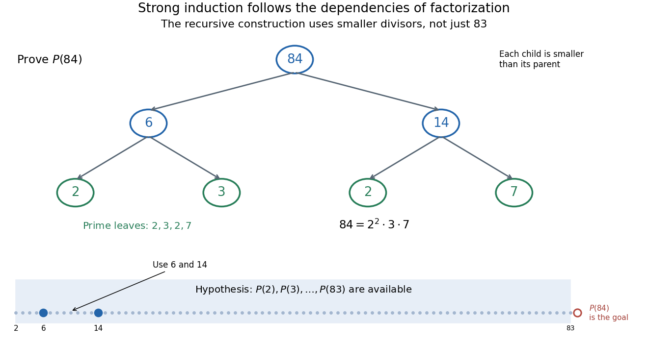
The step for 84 can use 6 and 14: the induction hypothesis covers both
. Original factorization tree , followed by and . Arrows show recursive dependencies toward smaller integers, rather than the order of increasing induction. The strip at the bottom marks the earlier cases available at the step for , with the required and highlighted. No use of the unproved case is permitted in the hypothesis. Details.
The same pattern explains the usefulness of strong induction for algorithm correctness. When a recursive procedure returns answers for smaller inputs, the induction hypothesis can justify those answers; the remaining task is to justify how the current call combines them. Strictly decreasing a nonnegative integer size measure establishes termination. Correctness also requires each call's conditions and its combination rule; termination alone does not make an algorithm correct.
Strong induction with four starting cases 2026-10-18
Consider a chosen packing problem: batches contain either four or seven identical items, with any nonnegative number of batches allowed. Which integer totals can be formed? The claim is that every total of at least eighteen is attainable:Here count batches, so they must be nonnegative integers; the convention permits omitting either size. Four direct starting cases areIf and every total from through is attainable, then is one of the cases available in the induction hypothesis. Add a batch of four to its representation to obtain . Thus the inductive step applies to every new total from onward. Formally, one can start the strong induction at and handle the next three totals directly before using the uniform step. The finite checks and the propagation together establish all totals, not merely those drawn below.
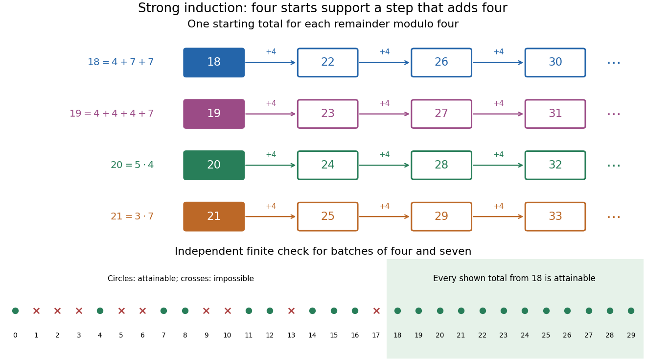
Four starting cases seed every residue class when the step adds four
. Original chosen batch sizes and . Colored rows follow ; ; ; and . Each arrow adds a batch of four. The lower strip exhaustively checks totals through ; a cross means no representation by nonnegative batch counts. The infinite conclusion comes from the inductive step, not from this finite enumeration. Details.
Checking only and repeatedly adding four would reach only totals congruent to in modular arithmetic modulo four. The four induction base cases supply all four residue classes. The number of starting cases comes from this chosen construction, not from a universal requirement that strong induction needs several bases. A different construction can need different starting information.
The threshold is sharp for these batch sizes. If , reducing modulo four gives , so . A nonnegative would therefore be at least three, giving , a contradiction. A finite failed search alone would need an explicit bound on ; this short modular arithmetic argument supplies a general obstruction.
For prescribed one-dimensional velocity , let , and expand the Lagrangian trajectory as . The Taylor expansion of gives and . Initial position requires andThe secular velocity is Stokes drift, even though the Eulerian time average vanishes. This fixed-time expansion requires and is not uniform once the secular displacement changes the phase by order unity.
Stern-Gerlach historical and modern interpretations Created 2026-10-18 Updated 2026-10-20
The 1922 interpretation concerned space quantization of atomic magnetic moments in the old quantum theory. The modern electron spin proposal came in 1925; the original observers did not identify intrinsic electron spin as the cause of their splitting. An orbital interpretation then seemed plausible, but the later spin explanation gives a different account of the same two-component evidence.[ref]
The Stern-Gerlach Experiment and the Electron Spin by Sandip Pakvasa. Pakvasa, pp. 1–3: original orbital interpretation, 1925 spin proposals and later reinterpretation
Modern atomic data assign neutral silver the ground state electron configuration and electronic term . The filled electron shells contribute zero net electronic angular momentum; the outer unpaired electron has orbital angular momentum , spin , and electronic total angular momentum . The magnetic quantum number has two values .[ref]
Atomic Data for Silver (Ag). Handbook of Basic Atomic Spectroscopic Data by Jean E. Sansonetti and William C. Martin; Ag I ground-state configuration and term; electronic J, distinct from isotope nuclear-spin rows
In the effective electronic description,The minus sign matters: for positive , the component with has negative electronic magnetic moment and deflects toward negative in our coordinates. Calling the upper spot “spin up” without specifying the magnetic field and channel calibration can therefore reverse the assignment. The total angular momentum operator here sums electronic orbital angular momentum and electronic spin; is not a claim that the atomic nucleus has no spin. Hyperfine structure and nuclear magnetic moments can require additional internal levels, so a two-channel electronic approximation must be justified for the field and resolution being used.
This is a neutral atomic beam, not a beam of free electrons. The deflected mass in the flight equations is the entire silver chemical atom; its dominant electronic magnetic moment supplies the state-dependent force. Replacing that atom by a free electron would also introduce the charged particle's Lorentz force and a different preparation problem. The ideal two-state model is useful because it isolates the connection between discrete internal components and spatially resolved outputs; it does not retroactively turn the 1922 deposit into a direct contemporary identification of intrinsic electron spin.
For an equally populated ideal pair of angular momentum eigenstates, the magnetic moment component takes two values, , and the displacements at fixed velocity are . Compare a specified classical alternative: every chemical atom carries a permanent magnetic moment of fixed magnitude , with independently isotropic initial orientations and no dissipative alignment. If , the sphere's area element is , so has a uniform distribution on . With precession preserving this component in the ideal geometry, the displacement fills the interval continuously. A pair of bands therefore tests allowed components rather than merely proving that silver is magnetic. Other classical preparation assumptions would be different models and must be stated.
To include finite instrumental width, choose a normalized Gaussian distributionwith standard deviation , representing a combined field-off spatial width. At fixed velocity the model probability density functions areEach has unit integral and zero mean; the different shapes, rather than a different average displacement, distinguish them. The discrete model has variance , whereas the classical model has variance . Their common mean also explains why the raw average landing position is insufficient to identify the internal quantum state.
Now choose a uniform distribution of forward velocities from to , explicitly as an example rather than the oven's actual distribution. Average either conditional probability density function over that interval. The positive-channel displacement ranges from to , since slower chemical atoms spend longer accelerating and drifting. The two components broaden into bands even though their internal magnetic moment values remain discrete. The corresponding classical profile continues to populate the center. The displayed strip darkness is proportional to predicted deposited number density, with equal total arrivals; it is not a photograph or a calibrated optical response of a developed film.
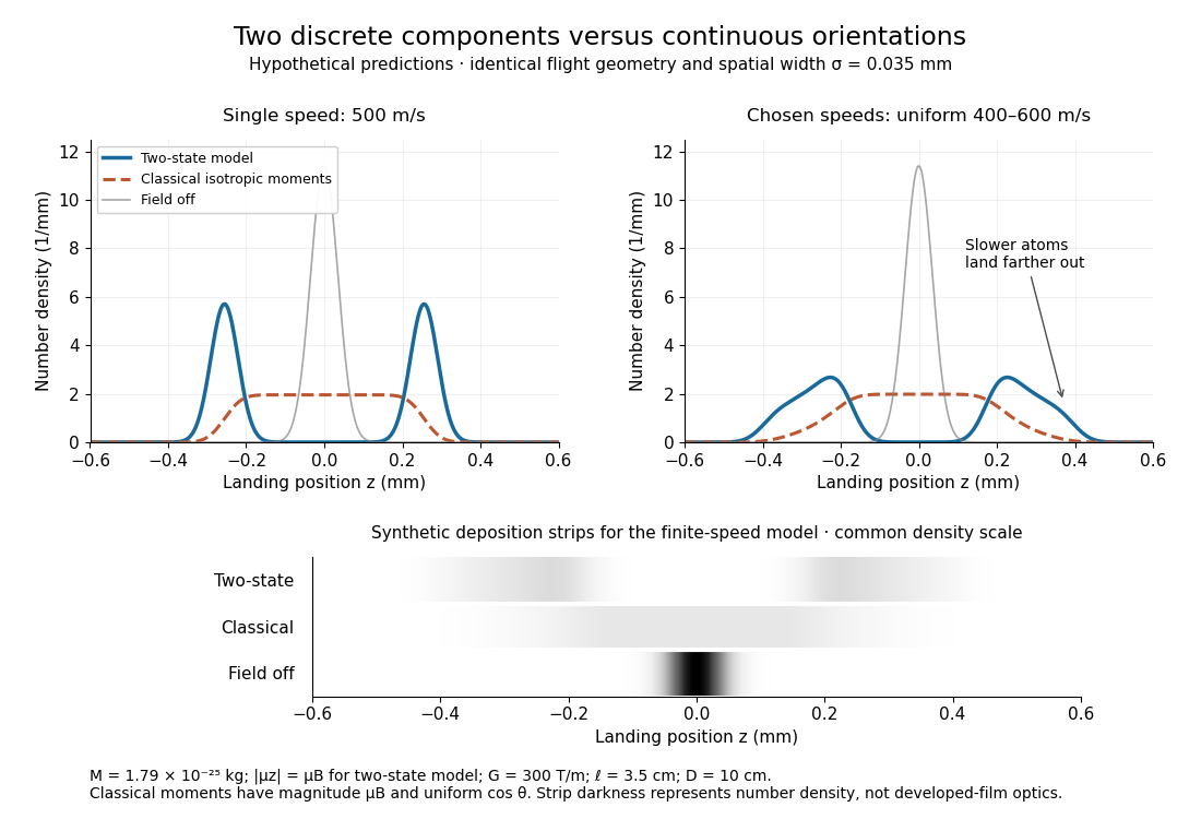
Discrete magnetic components and continuous classical deflections
. Original model predictions with the chosen flight parameters, comparing one forward speed with a finite speed interval. Both alternatives include the same Gaussian spatial width. Synthetic deposition strips use a common density scale; none of the curves or strips is measured data. Details.
Increasing the spatial width until it is comparable with can hide the two maxima. At fixed velocity, differentiating the two-state probability density function twice gives : the central minimum becomes a central maximum when . Conversely, a broad distribution of velocities need not create a new internal component: it spreads each existing component through the dependence. Further instrumental limits include collisions, aperture clipping of strongly deflected trajectories, asymmetric pole geometry, and nonlinear film development. Field-off widths and a mapped magnetic field gradient are needed to separate such effects. For a modern counting experiment, channel calibration and efficiency corrections belong to Stern-Gerlach expectation estimation; spatial separation alone does not supply those statistics.
Stern-Gerlach force and flight model 2026-10-18
Let the atomic beam travel along , with velocity , and let measure displacement along the dominant magnetic field gradient. For a fixed effective magnetic moment component , the magnetic dipole potential energy is . Taking its negative partial derivative givesA spatially uniform magnetic field can produce torque and Larmor precession, but cannot produce this translational separation. In a quantum state following a local internal energy eigenvalue , the more general expression is , with effective magnetic moment . Treating that moment as constant is an approximation with a physical regime, not an extra measured fact. Assume the local magnetic field direction stays nearly fixed across the sampled beam, and that internal states follow it without transitions, as in the adiabatic theorem. The scalar gradient model describes the beam's neighborhood; it omits the full magnetic field's transverse components and fringe regions.
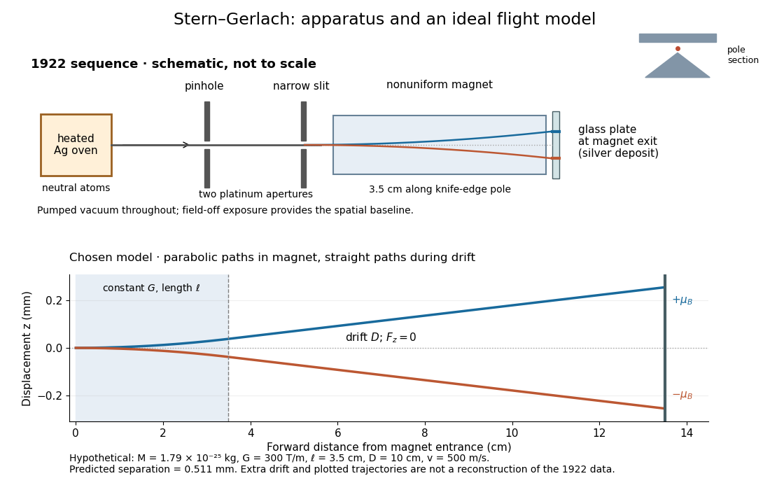
Assume a constant over magnet length , followed by a field-free drift . Neglect transverse motion at entry and changes in longitudinal velocity. Newton's second law gives transverse acceleration for whole-atom mass . The magnet transit time is , and the drift time is . The magnet supplies both a displacement and an exit transverse velocity:The contribution is motion with the acquired transverse velocity, not continued acceleration outside the magnet. For the plate-at-exit geometry, set . For a nonzero entrance transverse velocity , add . These terms show why initial collimation and flight geometry matter when inferring a magnetic moment from a deposit.
Choose hypothetical parameters , , , , and . Approximate the two effective magnetic moments by , where the Bohr magneton is . Then , and . The positive displacement is about inside the magnet plus during drift: , with full separation . These chosen values illustrate the model and are not reconstructed 1922 measurements.
The exit transverse velocity is only about , small compared with the chosen forward velocity; this checks the small-deflection assumption. Halving halves , doubling divides by four, and setting removes most of this example's separation. A real pole has fringe magnetic fields and a position-dependent gradient; these require a more complete trajectory calculation.
Stern-Gerlach apparatus in 1922 Created 2026-10-18 Updated 2026-10-25
In 1922, Otto Stern and Walther Gerlach used an electrically heated oven to emit neutral silver chemical atoms. Two platinum apertures, a pinhole and a slit – wide, supplied collimation. The beam passed along a knife-edge pole in a nonuniform magnetic field. At its end, a glass plate collected the condensed silver. Continuous pumping maintained vacuum; the thin deposit required development even after eight hours.[ref]
Der experimentelle Nachweis der Richtungsquantelung im Magnetfeld by Walther Gerlach and Otto Stern. Experimental setup, paragraphs 1–5; original 1922 paper in Martin Bauer's translation, PDF pp. 2–3
The field-off image established the undeflected slit width. A comparison put field-on and field-off deposits on the same plate. Microscopy revealed two deflected bands, no detectable central component, and broadening attributed to the velocity distribution. Alignment and distance from the knife-edge affected the pattern; precise magnetic field gradient measurements were still pending.[ref]
Der experimentelle Nachweis der Richtungsquantelung im Magnetfeld by Walther Gerlach and Otto Stern. Results, Figs. 2–5 and observations b–e; closing paragraph, PDF pp. 3–5
The apertures act as a collimator: they constrain the initial transverse positions and velocities, so a magnetic displacement can be distinguished from an initially broad beam. Vacuum reduces collisions that would destroy this preparation. Deposition integrates arrivals over the exposure; a darkened band is not a time-resolved record of individual chemical atoms. The field-off comparison tests whether the magnet changes the spatial distribution, while alignment checks address a geometric source of apparent asymmetry. Finite sensitivity qualifies the absence of a central deposit: it is an experimental upper limit, not a proof that exactly zero atoms landed there.


Display of the Stern-Gerlach apparatus at the University of Hamburg
. Photograph by Lesendes Okapi, 29 January 2019, CC BY-SA 4.0, via Wikimedia Commons. The display in the Institute of Physical Chemistry includes an apparatus arrangement and a plaque honouring Otto Stern. This photograph documents the later exhibition. Source.
Neutron Stern-Gerlach splitting Created 2026-10-18 Updated 2026-10-25
An electrically neutral neutron still has a magnetic moment . A collimated beam passing through an inhomogeneous magnetic field experiences the force derived from . In a region whose field axis is approximately fixed, a spin one-half neutron has two field-axis spin eigenstates, producing two allowed transverse forces and two separated beam components after a drift. A homogeneous field can cause Larmor precession but cannot separate positions through this force.
The neutron's negative gyromagnetic ratio interchanges which spin projection moves toward increasing field; it does not change the number of branches. An unpolarized beam gives equal ideal populations. A beam prepared in one field-axis eigenstate populates only one branch, so splitting into two observed spots presupposes both components and sufficient spatial resolution.
Adding a load to a spring-supported table shifts its static downward position by . If the load is deposited with negligible impulse and moves with the table, the moving mass is . Starting at the former equilibrium with zero velocity, an underdamped response isIts transient envelope decays over . Critical damping gives . A nonzero impact impulse changes the initial velocity and therefore the transient.
An exact teaching model makes the peak suppression explicit. Assume the narrowband field correlation separates as after delay compensation. Average each channel's light intensity over the same rectangular gate of duration . The two time integrals have triangular relative-delay weightIntegrating the Siegert relation against this weight givesThe factor is one for a selected polarization of waves and for two independent equally populated polarizations. The signal fraction uses mean stellar signal and independent additive background in each detector. The photon correlation loss and background model then supplies . This assumes no correlated sky background or electronic coupling.
For the original model , elementary integration givesThe area-based optical coherence time of this intensity envelope is . For , ; for , . With the chosen , , , and , and . At the stipulated disk gives approximately . A nearly unit measured can therefore conceal a substantial .
This rectangular-gate calculation specifies a counting model. An analog instrument's amplifier bandwidth and impulse response instead weight the fluctuations it actually passes; the Sirius amplifiers were bandpass devices. Both require measuring the response and calibrating the zero-baseline excess. When , , and the temporal response are unchanged, the ratio of excesses recovers :A sufficiently unresolved calibration source can supply the denominator; dividing the full values would give the wrong result. Narrower optical bandwidth lengthens optical coherence time, whereas wider usable electronic bandwidth can resolve faster fluctuations; these are distinct bandwidths. Background changes, unequal spectral responses, drift, or averaging over changing interferometric baselines can invalidate a common calibration. Resolving a disk means establishing a reproducible decline of calibrated correlation, supported by those controls.
Uniform-disk stellar visibility 2026-10-18
Stipulate a distant circular source of uniform angular brightness, full angular diameter in radians, and narrow optical bandwidth around wavelength . Distinct source patches emit independently. Assume each collector is small enough not to resolve the disk individually. For a sky offset from the disk centre, the baseline-dependent phase difference is , up to channel-sign convention. Summing independent patch contributions makes the equal-delay first-order optical coherence the normalized Fourier transform of angular brightness:Choose the horizontal coordinate along , put , and integrate along vertical chords of the disk:The imaginary part cancels between opposite chords. Here is the order-one Bessel function of the first kind. One way to obtain the last equality is to integrate the exponential's power series term by term on the finite disk. Equivalently the result is specified by the convergent seriesAt take the continuous limit ; starts as . This is why very short interferometric baselines give little leverage on angular diameter. Larger disks lose spatial optical coherence at shorter baselines.
The first positive zero of is , soThis is a full diameter convention. The angle must be converted before substitution: one arcsecond is radians, and one milliarcsecond, abbreviated mas, is arcseconds. For the stipulated and , and . At , the model gives and .
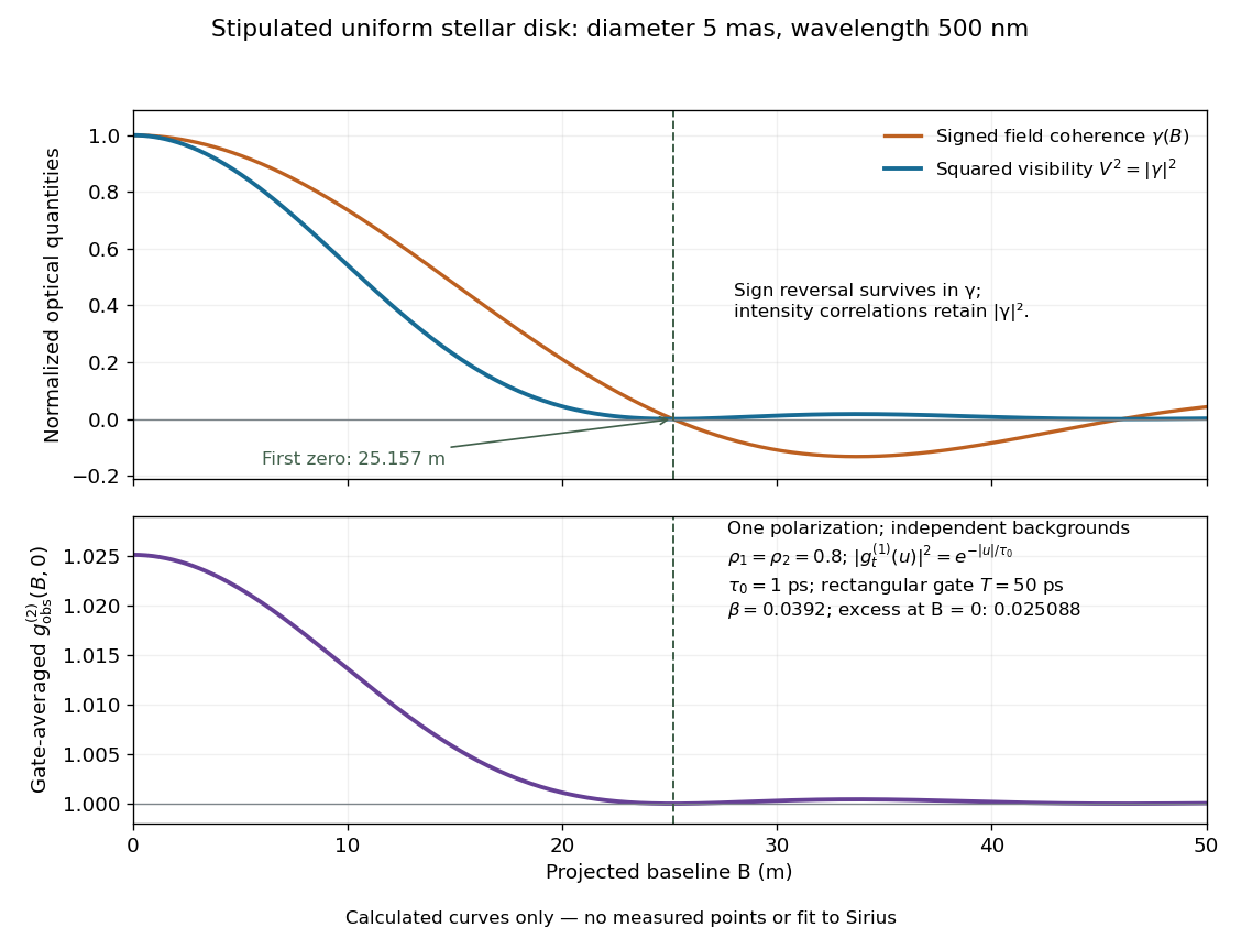
Stipulated uniform-disk model: signed field coherence, squared visibility and finite-gate intensity correlation versus interferometric baseline
. Original calculated curves for a 5-mas disk at 500 nm, with no measured points. The lower panel uses one polarization, independent signal fractions 0.8 in each channel, and the explicitly specified exponential temporal correlation and 50-ps gate below. It is not a fit to Sirius. Details.
Beyond , changes sign but stays nonnegative and develops weak further lobes. A single measured squared visibility can therefore match several angular diameters; sampling several interferometric baselines constrains the fit. Limb darkening, spectral averaging, or resolved collector apertures change the uniform-disk prediction. A uniform-disk diameter is a parameter of that brightness model; converting it to a physical stellar radius also requires distance and an appropriate brightness profile.
Siegert relation 2026-10-18
For one selected polarization of waves, write the detected complex fields as and their light intensities as , absorbing a common conversion constant. With stationary ensemble averages and nonzero , defineHere second-order optical coherence concerns distinct detector channels, with the corresponding normal ordering in the quantum formulation. Independent detection has . Subtracting the means gives the normalized covarianceThus multiplying raw photocurrents contains a large mean-product contribution; multiplying their fluctuations isolates the small excess. Independent detector shot noise does not supply a mean cross-channel excess, although it increases measurement uncertainty.
The displayed Siegert relation requires a zero-mean, jointly circular complex Gaussian random field, the usual chaotic thermal light model. Circular means invariance under a common arbitrary complex phase rotation; in particular . Apply the Gaussian moment pairing theorem to the real and imaginary parts:The remaining pairing vanishes by circularity. Division proves the Siegert relation. Gaussianity is an assumption about fourth moments, not a consequence of merely measuring first-order optical coherence; a coherent state or photon antibunching cannot be interpreted by this thermal formula.
For equal-intensity beams combined in a common optical mode with matched wave polarizations, interferometric visibility is . Consequently ideal thermal stellar intensity interferometry measures , while the full includes the independent-count reference one. Unpolarized thermal light with two independent equally populated wave polarizations has half this excess: adding their covariances doubles the numerator while multiplying total means quadruples the denominator. Finite detector response further suppresses the peak and must be calibrated.[ref]
Spatial intensity interferometry on three bright stars by William Guerin and others. Guerin and others, Spatial intensity interferometry on three bright stars, arXiv:1805.06653v2 (13 August 2018), §§2.1–2.3: normalized correlation, thermal contrast and temporal-response calibration
Sirius intensity interferometry experiment 2026-10-18
In their 1956 Sirius report, Robert Hanbury Brown and Richard Q. Twiss used two 1.56-m searchlight reflectors feeding photomultipliers. The photocurrent fluctuations passed through 5–45-MHz amplifiers; an adjustable delay aligned arrival times. A linear mixer multiplied the outputs; an integrating motor accumulated their product. A second motor monitored its root-mean-square fluctuation to control gain changes. Separate lamps illuminated capped photomultipliers before and after observations to test electronic coupling and drift; blank-sky runs tested correlated sky background. They fitted a uniformly bright disk and an unknown zero-baseline scale to relative correlations at different interferometric baselines. Broadband response and possible baseline-dependent systematic errors limited the diameter inference.[ref]
A Test of a New Type of Stellar Interferometer on Sirius by Robert Hanbury Brown and Richard Quentin Twiss. pp. 1046–1048: reflectors, delay/correlator, lamp and sky controls, relative-baseline disk fit
This astronomical test extends the preceding laboratory Hanbury Brown and Twiss effect to two independently collected samples of a star. The historical motor reading was an instrument-specific correlation statistic. It should not be identified numerically with the normalized below without the corresponding measurement calibration.
False alarm rate Created 2026-10-18 Updated 2026-11-05
The expected rate of detections exceeding a stated threshold under a specified background-only model. A time rate and a per-trial significance level require different normalizations.
Malmquist bias 2026-10-18
Standardizable candle 2026-10-18
A standardizable candle has a predictable absolute magnitude after correcting measured source properties, rather than identical intrinsic brightness for every object. Type Ia supernova cosmology uses light curve shape and colour for this purpose.
Blocking pair in stable matching 2026-10-18
An acceptable unused edge whose endpoints both prefer each other to their partners in a matching in a graph, treating every acceptable partner as preferable to being unmatched. A stable matching has no such edge. In the worked example, blocks even though already has its first choice.
For a real scalar height field, integration by parts givesThe bulk expression is even under time reversal. The original density is not pointwise even, but changes by a total divergence; its stationary equation is time-reversal invariant. The first-order diffusion equation selected by zero residual is not invariant under ordinary time reversal at fixed positive . Boundary conditions or the probabilistic interpretation can distinguish the two time directions even when the higher-order stationary equation does not.
Helium-3 pair order parameter 2026-10-18
For a simple spin-triplet p-wave pairing description, let the matrix , with complex number entries, map an orbital direction on the Fermi surface into a triplet gap vector . The indices refer to spin and orbital components. A scalar amplitude cannot retain all these relative orientations. Anthony James Leggett's account connects that extra structure to the magnetic responses of the different phases.[ref]
Nobel Lecture: Superfluid 3He: the early days as seen by a theorist by Anthony James Leggett. pp.1004–1008, broken spin-orbit symmetry and pairing-state response
Here are two explicit idealizations, with a common positive scale and an overall quantum phase omitted. They show how odd orbital pairing can have either nodes or an isotropic gap. They do not calculate which state has the lower Helmholtz free energy.
Spin-flip scattering Created 2026-10-18 Updated 2026-11-05
Spin-flip scattering is a collision or scattering event that changes a particle's spin projection along a specified quantization axis. For electrons, coupling to another magnetic moment or coupling of motion to spin through spin-orbit coupling can transfer angular momentum between the electron spin and other degrees of freedom.
Repeated events can relax a nonequilibrium spin polarization, making spin-flip scattering one mechanism of spin relaxation. The axis and state basis must be stated: in a spin-orbit-coupled material, the propagating energy eigenstates need not be pure up or down states along one fixed axis. Conversely, decay of transverse coherence need not imply flips; different precession phases can cancel the ensemble's transverse signal while individual spin populations remain unchanged.
There are unlisted articles, also show them or only show them.