
Nuclear pairing 2026-10-18
Correlations that favor pairs of like nucleons coupled to zero total angular momentum in the simplest spherical picture. They help explain why an unpaired nucleon often dominates an odd nucleus's spin, and why neighboring nuclear separation energies show an odd-even staggering. Nuclear pairing belongs to the residual-interaction physics beyond merely filling independent energy levels. Mixing different occupations and deformation can also be necessary; the closed-core picture is most useful near suitable nuclear shell closures.
Nuclear separation energy 2026-10-18
The energy needed to remove specified nucleons from a bound atomic nucleus in its ground state. It compares neighboring nuclear masses, and so can reveal a nuclear shell closure more clearly than a smoothly varying total nuclear binding energy.
Nuclear spin-orbit splitting 2026-10-18
The splitting of one-nucleon energy levels by their spin-orbit interaction. With , the identity gives, in a state of definite ,The second branch requires . For the illustrative Hamiltonian operator with , the shifts are and . Thus the strong negative coefficient lowers the aligned branch. Its capacity is ; the raised partner holds . Together they still hold identical nucleons: the interaction rearranges states rather than creating them.
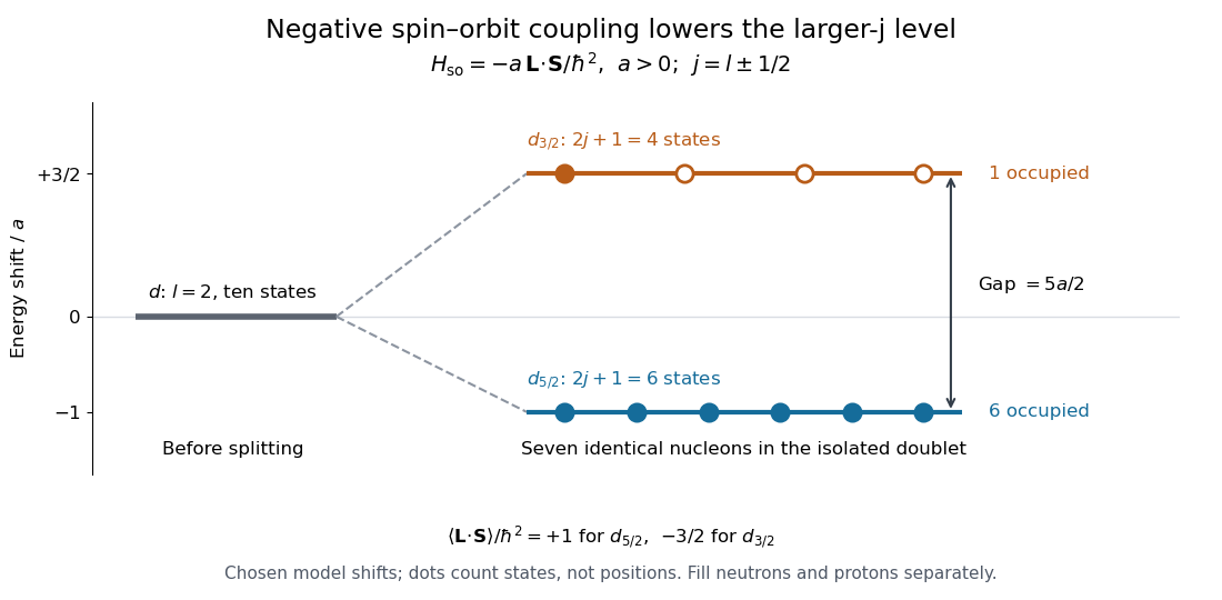

In this example the and shifts are and , respectively, so the gap is . The capacity-weighted mean shift vanishes:This is a useful check on both the sign and state counting. A seventh identical particle cannot occupy another substate of the already full lower level. In a real atomic nucleus, other radial and orbital angular momentum levels can interleave with this doublet, and a radial coupling need not give the same effective for every orbital.
Magic number 2026-10-18
A proton number or neutron number associated with a pronounced nuclear shell closure. The traditional sequence isThese count either species separately, rather than their sum . Calling a number magic summarizes a structural pattern; it does not promise that every isotope at that number is equally stable.
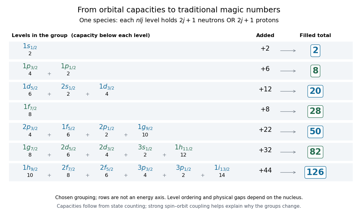
Counting states between traditional nuclear shell closures
. Original capacity diagram for a chosen spherical level scheme. Each orbital contributes states for one species. Rows show groups and cumulative totals, not measured energies or a universal ordering within each group. Details.
For example, in the chosen scheme the -particle core plus the eight substates of gives . The next group contributes , giving . The following two groups contribute and , giving and . Counting verifies the capacities once the grouping has been chosen; it does not establish the physical energy gaps that justify that grouping.
Nuclear mean field 2026-10-18
An effective one-nucleon potential energy representing the average influence of the other nucleons. The nuclear shell model treats motion in this field first, then includes residual interactions. The field experienced by a proton also includes the repulsive Coulomb potential; proton and neutron energy levels need not have identical spacings.
Nuclear shell 2026-10-18
A nuclear shell groups single-particle energy levels for protons or neutrons in a nuclear mean field. Filling all states below a sufficiently large gap gives a nuclear shell closure. These shells describe quantum-state occupation rather than thin spatial layers. Their discrete filling effects explain departures from the smooth semi-empirical mass formula.
Single-particle nuclear magnetic moment Created 2026-10-18 Updated 2026-10-20
In the simplest nuclear shell model of an odd-mass number nucleus, paired nucleons contribute zero total angular momentum and magnetic dipole moment. The last unpaired nucleon supplies the nuclear spin and the stretched-state moment , where is the Landé g-factor and the nuclear magneton.
Using addition of angular momentum with givesFor , this reduces to . For , it givesThe free-nucleon orbital factors are for a proton and for a neutron. Residual nuclear interactions and configuration mixing can shift measured moments away from this ideal prediction. A single hole in an otherwise closed shell has the same stretched-state moment as a particle in that shell: removing the particle leaves total and moment .
Nuclear rotational spectroscopy evidence Created 2026-10-18 Updated 2026-10-20
Aage Niels Bohr's 1975 lecture presents a plutonium spectrum deduced from the fine structure of alpha decay of curium . The readout was decay-line energy; the comparison fixed the rotor scale from the first excitation and tested the remaining levels against . The lecture reports spectroscopy, rather than a laboratory setup operated by its author.[ref]
Rotational Motion in Nuclei by Aage Niels Bohr. p. 217, Fig. 3 caption, plutonium spectrum and one-scale comparison
His measured erbium band has excitation energies , , , and for . The same lecture analyzes interband electric quadrupole transitions, adding tests beyond level positions.[ref]
Rotational Motion in Nuclei by Aage Niels Bohr. p. 225, Fig. 9 measured levels and following discussion of Fig. 10 transition matrix elements
Using those first two excitations gives , close to the ideal , and distinct from the ideal harmonic value . Fixing the rotor scale with predicts at and at . The measured values lie about and below these predictions. This is a useful limit of the simple model: the pattern supports a rotational interpretation while revealing departures from constant inertia. It does not by itself determine a unique nuclear charge distribution. Reconstructing a level scheme also requires assigning which transitions connect which states; raw peak positions alone do not provide all spins, parities or transition strengths.
Nuclear elastic electron scattering kinematics Created 2026-10-18 Updated 2026-10-20
An elastic scattering event leaves the nuclear internal quantum state unchanged while transferring energy to its motion. Let a target of mass initially be at rest. Neglect the electron rest mass, but retain relativistic target recoil. Conservation of momentum and conservation of relativistic energy giveEliminating yields and henceThe static relation follows only when is negligible. For small recoil, ; this last approximation is nonrelativistic for the recoiling nucleus, not for the incident electron. The invariant spacelike transfer, expressed in energy-squared units, isso and the spatial inverse length coincide only in the static limit. Recoil kinematics alone does not correct the static differential scattering cross-section: a finite-mass target also changes its kinematic prefactor and the appropriate current matrix elements.
Pion decay at rest in emulsion 2026-10-18
Cecil Frank Powell's 1950 lecture illustrates the successive decays of pions and muons through their tracks and explains why the nearly fixed secondary muon range, allowing for range straggling, supports a single neutral decay partner. He describes its identification as a neutrino tentatively. The neutral particle itself leaves no recorded track. He contrasts this decay with the nuclear reactions caused by stopped negative pions, connecting the latter with the nuclear force.[ref]
Here is a modern special relativity derivation for the dominant leptonic pion decay, assuming a free pion at rest, a massless muon neutrino, and no emitted photon. Write and for the pion and muon masses. By conservation of momentum the daughter momenta are opposite with equal magnitude . By conservation of energy and the energy–momentum relation,Substitute , square, and cancel . This givesThe resulting is fixed, although the muon's direction is not set by the incoming stopping track. Thus the kink angle relative to that earlier track is not the angle between the two daughters: in the pion rest frame, the daughters are back to back. A neutral-partner arrow in a diagram represents inferred momentum, not an observed string of grains.
For an original calculation, adopt rounded input values and . They give , and . Their sum satisfies . These are rounded calculation inputs and outputs, not a fit to the 1947 plates.
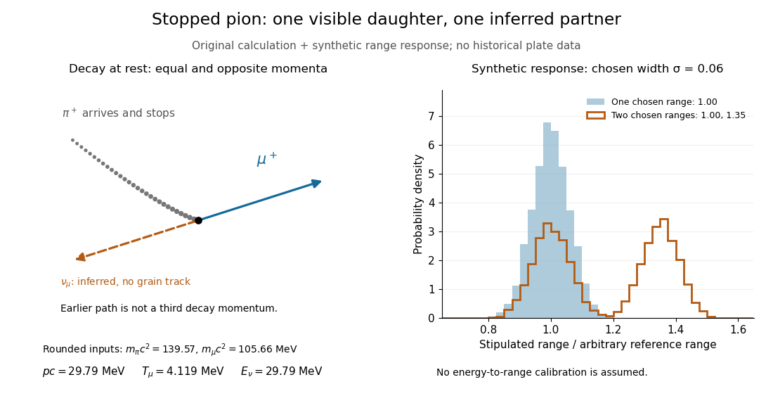

At fixed material and particle identity, a fixed initial kinetic energy suggests a narrow particle range distribution broadened by range straggling and measurement uncertainty. The synthetic example convolves a single chosen range with a normal distribution; a second example superposes two such chosen ranges. It explains why repeated comparable stopping distances can be informative, without pretending to extract a historical spectrum.
The decay equations do not identify the neutral partner as a neutrino on their own: a massless photon would satisfy the same energy and momentum equations. Nor does any isolated kink establish the pion's identity. The inference gains force from calibrated particle range, track grain density, repeated decay patterns and independent particle properties. Historical particle names should not obscure the distinction: a muon is a lepton, whereas a pion is a meson.
Track grain density 2026-10-18
The track grain density is the number of resolved developed grains along reconstructed track length , divided by . It is a response variable, not a universal conversion from darkness to energy. Overlapping developed grains, exposure fading, processing and optical spatial resolution can all change what is counted. Calibration must use comparable material and viewing conditions.
Cesare Lattes specifically recalls distinguishing meson tracks from proton tracks using their greater deflection by scattering and changing track grain density toward the stopping point. He also recounts a secondary track that left the coating, requiring extrapolation rather than a directly measured stopping distance.[ref]
Meu Trabalho em Física de Mésons com Emulsões Nucleares by Cesare Mansueto Giulio Lattes. 1984 recollection, paragraph beginning “Devo adicionar”: scattering, grain density and an escaping secondary; no numerical grain count is reported here
For a candidate joined track, the useful questions are whether both branches actually meet in depth, whether the incoming branch is consistent with stopping there, and whether the outgoing branch has the expected particle range and track grain density. A visible change of direction alone cannot distinguish a decay from scattering or an accidental crossing. Examining successive focal depths tests a projected crossing; comparison with ordinary stopping tracks tests the identification. These are measurement checks, not a claim that the original plates provided time-resolved movies.
A nuclear emulsion integrates exposure over time. It does not by itself supply the time between two apparently joined branches. Finite spatial resolution also limits how tightly one can establish their common origin: developed marks and the microscope response are much larger than a subatomic particle. There is no single resolution number applicable to every emulsion, developer and optical arrangement.
Emulsion range measurement 2026-10-18
An emulsion range measurement follows a stopping charged particle through the coating to estimate its complete particle range. A projected length on one image can underestimate the distance travelled. In an original geometry example, a straight segment with projected length and corrected depth change has lengthUsing the projection alone would underestimate this length by . A bent track requires a sum over reconstructed segments. These are stipulated coordinates, not measurements of a historical track.
Suppose photographic processing contracts the coating only in depth, with shrinkage ratio . Then an observed depth difference corresponds to . For , an observed becomes the used above. This correction assumes uniform contraction and unchanged lateral dimensions; it cannot repair a track that leaves the coating before stopping.
A simple continuous-loss model connects particle range to kinetic energy through stopping power :This describes the mean trend for a specified particle and material. Fluctuating energy loss produces a spread of stopping distances, called range straggling. An exit point supplies only a lower bound on particle range. Consequently, a narrow distribution from fully contained tracks and one assembled by treating exits as stops answer different questions.
Spectroscopic nuclear quadrupole moment 2026-10-18
The laboratory expectation value of the axial electric quadrupole moment in the stretched nuclear quantum state ; is the laboratory component of total angular momentum. It differs from the intrinsic nuclear quadrupole moment . In an axial nuclear rotational band with , projection onto definite angular momentum givesHere denotes the component of total angular momentum along the intrinsic symmetry axis. Consequently a positive for a prolate spheroid corresponds to a negative in this model. The sign of the laboratory moment alone must be interpreted together with the band assignment.
The result has a short symmetry explanation. A spin-zero state has no preferred spatial direction. Its second charge moments satisfy , so . Equivalently, averaging an intrinsic axis uniformly over directions gives , where is a Legendre polynomial. This is a statement about a quantum expectation value, not a classical picture of a spinning object sweeping through orientations.
For an independent check of the sign, the , rotor orientation probability is proportional to , using a spherical harmonic. With ,A zero static laboratory moment does not make every quadrupole observable zero. With electric multipole operator , define the reduced transition strength using a reduced matrix element:In the axial rotor, angular projection gives and . The factor of five is the ratio of the numbers of magnetic substates. Thus an electric quadrupole transition can reveal collective deformation even when . These strengths determine within the model; their squares alone cannot distinguish its sign.
Intrinsic nuclear quadrupole moment 2026-10-18
The axial electric quadrupole moment of an intrinsic nuclear charge distribution, with the origin at its center and the axis along its symmetry axis:This convention includes electric charge in ; a tabulated moment divided by the elementary charge instead has units of area. For the uniform spheroid, mapping a uniform unit ball to gives and , soThe formula explains the signs in the figure. It measures an anisotropy of the nuclear charge distribution, rather than counting individual nucleons on a surface. An illustrative choice gives , and , while preserving exactly.
James Rainwater's lecture contrasts measured laboratory electric quadrupole moments with intrinsic moments inferred through Coulomb excitation, including even-even nuclei. Extracting intrinsic shape therefore uses a nuclear model, rather than equating every measured moment to .[ref]
Background for the Spheroidal Nuclear Model Proposal by James Rainwater. p. 266, Fig. 4 and preceding Coulomb-excitation discussion
Nuclear charge form factor 2026-10-18
In the static charge density model, define the normalized Fourier transformHere is the spatial momentum transfer divided by the reduced Planck constant: has units of inverse length. Physical momentum transfer is . We keep and the speed of light explicit; compute , expressing the numerator in and in , to obtain in inverse femtometres. The spatial is distinct from the invariant four-momentum transfer used in relativistic scattering cross-sections.
For spherical symmetry, take the polar axis along and use spherical coordinates. With the cosine of the polar angle,Every radial shell contributes an amplitude. At all shells add with the same sign; at larger their contributions can cancel. This cancellation is the origin of a diffraction minimum in the nuclear charge form factor, rather than an absence of electric charge in the nucleus.
The static Fourier transform interpretation is appropriate for the nuclear model and kinematic regime specified here. A fully relativistic composite system requires frame and current conventions; its electric form factor is not universally the transform of a frame-independent three-dimensional charge density.
Nuclear charge radius 2026-10-18
The root mean square radius of a nuclear charge distribution, referred to its center. Define its charge-weighted second moment byFor a spherical charge density with finite fourth moment, insert the Taylor series into the nuclear charge form factor:Thus a radius is a low-momentum transfer slope, not necessarily the position of a sharp edge. In this real static model,The factor of two between the slopes of and matters when interpreting a differential scattering cross-section. A proton charge radius is the corresponding size concept for the proton; the spatial arrangement of many nucleons introduces an additional scale in a heavier atomic nucleus.
Hofstadter nuclear electron scattering experiment Created 2026-10-18 Updated 2026-10-20
Robert Hofstadter's Stanford installation selected electrons up to . Magnetic spectrometer scans counted shielded Lucite Cherenkov radiation pulses per monitor charge. Carbon-12 at and resolved elastic scattering and inelastic scattering ( excitation). Calibration used forward-beam energy, hydrogen nuclear recoil and carbon-12 energy levels. Closed entrance slits checked background.[ref]
Electron Scattering and Nuclear Structure by Robert Hofstadter. §III(b)(1), pp. 222–223, Fig. 11; §IV(a), pp. 227–231, Figs. 14–17
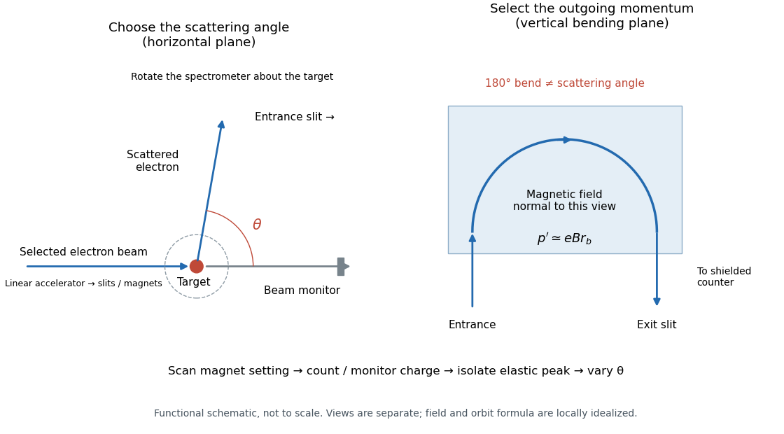

The key distinction is between an electron counter and an energy measurement. Here the counter registers particles admitted by the magnetic spectrometer; changing its magnetic field selects another outgoing momentum. A peak is therefore reconstructed from a scan, rather than read as one pulse whose height equals the scattered electron energy. Dividing counts by monitored incident electric charge compensates for changes in beam intensity. A peak's height alone is insufficient: its area and the instrument's accepted momentum interval determine the selected yield.
An inelastic scattering peak corresponds to a different final nuclear quantum state, so including it in the elastic scattering yield would answer a different structural question. Conversely, finite energy resolution can hide sufficiently nearby excitations beneath an apparent elastic scattering peak. Background subtraction, target-loss corrections, angular acceptance and counter efficiency all enter before counts become a differential scattering cross-section. A dip in uncorrected counts is therefore not automatically a zero of a nuclear charge form factor.
Two-parameter Fermi nuclear charge distribution Created 2026-10-18 Updated 2026-10-24
A common spherical model of a heavy nuclear charge distribution uses a half-density radius and surface diffuseness . The normalization is fixed by . The 90%-to-10% surface thickness is : solve and and subtract the two radii. Typical fits have an approximately constant surface thickness and a radius scaling roughly as the cube root of mass number. This is a spatial density model, not an assertion of a thermal Fermi-Dirac distribution for nuclear positions.
Semi-empirical mass formula 2026-10-18
The semi-empirical mass formula approximates nuclear binding energy using volume, surface, electrostatic, neutron-proton asymmetry, and nuclear pairing contributions. At fixed mass number, its quadratic dependence on atomic number gives a nuclear mass parabola. It describes broad trends and does not resolve individual nuclear shell effects.
Binding energy per nucleon Created 2026-10-18 Updated 2026-10-20
Binding energy per nucleon divides conventional positive nuclear binding energy by mass number. Typical well-bound nuclei have values of order , and the broad maximum lies near iron-group nuclei. A mass correction added to free-nucleon masses instead has the opposite sign, .
There are unlisted articles, also show them or only show them.