
Grism Created 2026-10-18 Updated 2026-11-05
A grism combines an optical prism with a diffraction grating. Their angular deviations can be chosen to cancel at a selected wavelength, while neighboring wavelengths emerge in different directions. This lets an instrument introduce spectral dispersion with approximately straight-through propagation at its design wavelength.
Inserting the grism into an imaging beam turns compact object images into dispersed optical spectra. The cancellation is wavelength-specific and order-specific: overlapping spectra and other diffraction orders remain potential sources of confusion. An optical filter can restrict the recorded band.
Mirror 2026-10-18
A mirror redirects light according to the law of reflection. Its orientation determines the reflected beam direction in an interferometer.
Optical cavity Created 2026-10-18 Updated 2026-10-20
An optical cavity supports optical fields whose phases and spatial profiles reproduce themselves after a round trip through its reflecting or guiding elements. Its resonance conditions include propagation and reflection phases. A cavity bounded by two plane mirrors is a simple example; Fabry–Pérot resonance spacing describes the frequency intervals of an ideal two-mirror arrangement.
Circular dichroism 2026-10-18
Circular dichroism is unequal absorption of opposite circular polarizations. It can produce elliptical polarization; it is the absorptive response related to optical rotation, rather than the same measured quantity.
Matrix mechanics Created 2026-10-18 Updated 2026-10-20
Matrix mechanics represents an observable by an array of matrix elements between chosen quantum states. In an orthonormal basis of energy eigenstates, each a stationary state, the diagonal entries of the Hamiltonian operator are the energy levels; off-diagonal entries of other observables describe couplings between those states. The same array can therefore answer two different questions: which values can a measurement return, and which pairs of energy eigenstates can a specified interaction connect? The eigenvalues answer the first question; the relevant matrix elements, together with the energy differences, answer the second.
This makes linear algebra a practical language for atomic physics. One can calculate energy levels, electric-dipole selection rules and probability amplitudes for transitions without assigning an electron an unobserved classical orbit. The three-state example below separates a missing optical coupling from a missing energy level; the finite oscillator commutator boundary defect explains why a finite array requires care when approximating a quantum harmonic oscillator.
Hash table probe 2026-10-18
One inspection of an array slot during an open addressing operation. Its array index follows the chosen probing rule; its contents determine whether to continue, return a matching hash table record, or establish absence.
Tombstone in open addressing 2026-10-18
A deleted-slot marker in open addressing. Lookup continues past it because a hash collision may have displaced a match further along. Linear probing can reuse the slot for insertion after checking for an existing equal key. A genuinely empty slot can terminate lookup; this marker cannot.[ref]
5.2 LinearHashTable: Linear Probing. Open Data Structures: An Introduction by Pat Morin; section 5.2, find, add, remove, and correctness paragraph distinguishing del from nil
Delete hash table key from the original eight-slot example. Writing
E into array index makes lookup of inspect and incorrectly report absence, although its hash table record remains at . Writing D instead makes lookup pass and reach , returning after three hash table probes. The deleted slot must remember that the search route once continued through it.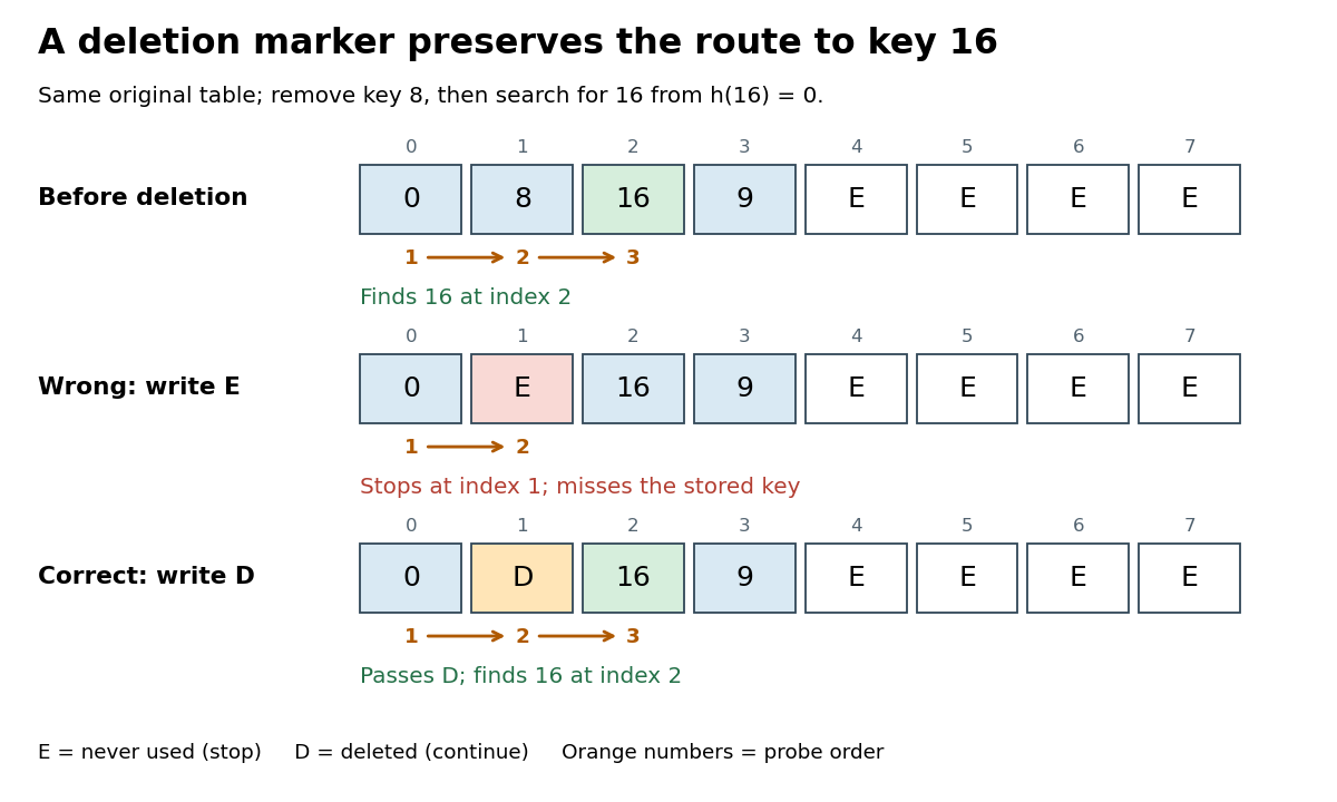
Deleting to an empty slot breaks lookup; a tombstone in open addressing preserves the search route
. Original deterministic comparison: the middle and lower rows are alternative deletions from the top row. E means never used and stops lookup; D means deleted and lets lookup continue. Orange numbers give the hash table probe order for hash table key . Details.
A short algorithm correctness proof uses this invariant: no never-used slot precedes a stored hash table key along its linear probing route. Initially the claim is vacuous. Insertion places a new hash table record no later than the first
E, possibly at an earlier D, and cannot create an E before another stored hash table record. Replacing a value leaves all slots occupied as before. Deletion to D also creates no E. By mathematical induction over operations, the invariant persists, so stopping lookup at E is sound. Deletion directly to E invalidates that argument, as the diagram shows.To implement the hash table map operation
put(k,v) in one bounded scan, remember the first D encountered, but keep checking occupied hash table keys. A later key equality match means replace that hash table record's value and stop. Only after reaching E, or completing hash table probes, is absence established. Then insert at the remembered D, if any; otherwise use the stopping E. If all slots are occupied and no match exists, report full or rebuild before trying again. Merely finding D is not permission to create a second equal hash table key.[ref]Continue from the correctly deleted example, with hash table keys at array indices and
D at . put(16,Z) examines and updates the value at , leaving deleted and retaining three live hash table records. Inserting immediately at would instead create two copies of . Now put(24,W) examines , proves absence at E, and places the new hash table record at the remembered array index . The hash table load factor rises from to ; reusing D avoids extending the linear probing cluster to .For a boundary case, fill all eight slots with hash table keys and then delete all eight to
D. The live hash table load factor is zero, but absent lookup of still needs eight hash table probes. put(16,C) also checks eight slots before reusing the first D, at array index . A loop that waits indefinitely for E would never finish in this state. Rebuilding from the live hash table records into a fresh array removes each tombstone in open addressing and restores never-used stopping slots.[ref]5.2 LinearHashTable: Linear Probing. Open Data Structures: An Introduction by Pat Morin; Section 5.2, resize: reinsert live elements and reset the non-nil count to the live count
Linear probing 2026-10-18
An open addressing probe rule that visits modulo , using modular arithmetic, until a matching record or an appropriate stopping slot is found.[ref]
Lecture 10: Hashing III: Open Addressing. 6.006 Introduction to Algorithms, Fall 2011 by Massachusetts Institute of Technology, 6.006 course staff; Lecture 10: Hashing III: Open Addressing, p. 3, Linear Probing formula
For capacity , the hash table probe numbered , starting at zero, inspects the array indexThe hash function gives the first array index. Each subsequent hash table probe moves one slot forward, wrapping from to by modular arithmetic. Keep the hash function and key equality fixed while hash table records are stored.
Use three distinguishable slot states: occupied by a live hash table record; never used since initialization or rebuilding, written
E; or deleted, written D, a tombstone in open addressing. Lookup compares occupied hash table keys using key equality, stops at E, and continues past D.[ref]5.2 LinearHashTable: Linear Probing. Open Data Structures: An Introduction by Pat Morin; Section 5.2, three entry types and find: nil stops lookup, del does not
For an original example, take an eight-slot array, integer hash table keys, and the hash function . Start with all slots
E and insert the hash table records in that order. The insertion hash table probe traces, expressed as array indices, areThe resulting array holds hash table keys at array indices , with E in the other four slots. The first three hash table keys have the same initial array index, a hash collision; the fourth begins at but joins the same linear probing cluster. Lookup of examines array indices , rejecting before returning . Lookup of absent examines , including the stopping E: five hash table probes for a hash table load factor .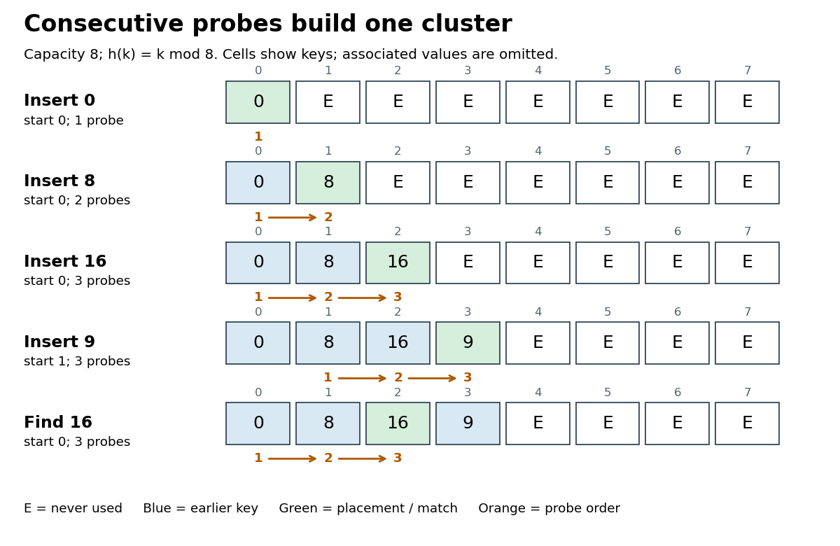

Bound lookup to at most hash table probes, even if no
E remains. For algorithm termination, the first array indices are distinct: equality of and implies that divides by modular arithmetic, and forces . They therefore cover the entire finite set of slots exactly once. If no occupied hash table key matches and no E is encountered, exhausting these hash table probes establishes absence; wrapping around again supplies no new information.[ref]Lecture 10: Hashing III: Open Addressing. 6.006 Introduction to Algorithms, Fall 2011 by Massachusetts Institute of Technology, 6.006 course staff; Lecture 10: Hashing III: Open Addressing, pp. 1–2, probe permutation requirement and Search loop with m trials
The attraction is a compact array and a simple hash table probe rule. Consecutive slots can benefit from spatial locality, although actual memory cache behavior depends on representation and hardware. Correctness rests on preserving the search route; speed depends on how long that route becomes. The linear probing cluster below explains why even a moderate hash table load factor gives no universal constant lookup bound.
Nuclear tensor force 2026-10-18
The linear operator couples nucleon spin orientations to their separation direction . Here are Pauli matrices. A scalar radial potential energy alone omits this directional dependence.
Work by Oliver Cecil Simpson 2026-10-18
Work by Ole Knudsen 2026-10-18
Radio astronomy 2026-10-18
Radio astronomy studies celestial sources through their radio waves. The long wavelengths make angular resolution expensive: a filled telescope of diameter has a characteristic diffraction scale of order . Aperture synthesis instead combines measurements from separated antennas, using their separations to measure fine structure while their individual collecting areas determine how much radiation they receive. A kilometre-wide arrangement of small antennas does not collect the power intercepted by a filled kilometre-wide dish.
X-ray astronomy Created 2026-10-18 Updated 2026-10-20
X-ray astronomy infers the properties of celestial sources from their X-rays. It requires instruments above the strongly absorbing layers of Earth's terrestrial atmosphere. Riccardo Giacconi's 2002 Nobel lecture connects the early rocket detections to later grazing-incidence X-ray optics, which collect photons over a large entrance area onto a small detector.[ref]
The Dawn of X-Ray Astronomy by Riccardo Giacconi. The Dawn of X-Ray Astronomy, introduction and section 4, pp. 123–124
The measurement is an inverse problem: a count rate mixes incident photon arrival rate, detector response, and background. A point-like astronomical source produces a direction-dependent excess as the instrument scans; diffuse X-ray background contributes over many directions. Neither a count excess nor a narrow feature by itself determines the emission mechanism. The useful progression is from detecting an excess, to locating it, to measuring its spectrum and light curve.
Backward error 2026-10-18
A backward error measures a perturbation of the input data for which the computed result is an exact solution of the perturbed problem. Specify which data may change and which norm measures the perturbation. For a linear system , holding fixed gives , the negative linear-system residual. The corresponding forward error also depends on the condition number.
Forward error 2026-10-18
The forward error is the difference between a computed result and the exact result for the original data. Its size can be measured by a norm, or relative to when . A linear-system residual measures the equation imbalance instead; the condition number relates that imbalance to the forward error.
Significant figures Created 2026-10-18 Updated 2026-10-20
In numerical analysis, significant figures record how many meaningful digits are retained in a written numerical value. Leading zeros locate the decimal point rather than adding precision: and each have two significant figures. Trailing zeros may require an explicit convention to distinguish measured precision from positional notation.
Nuclear de-excitation Created 2026-10-18 Updated 2026-10-20
Nuclear de-excitation is a transition from a higher to a lower nuclear energy level. It can transfer energy to an emitted gamma ray or to an atomic electron through internal conversion, among other channels when thresholds permit.
Nuclear level scheme 2026-10-18
A nuclear level scheme represents nuclear energy levels and transitions among them. Gamma ray energies constrain pairwise differences; emission counts and coincidence measurements help resolve different schemes having the same difference multiset.
The 1948 empirical synthesis preceded the 1949 strong spin-orbit interaction proposals. Johannes Hans Daniel Jensen recalled developing that idea in a discussion with colleagues, independently of Maria Goeppert Mayer's work; their shared problem was to account for the observed magic numbers and spins.[ref]
Glimpses at the History of the Nuclear Structure Theory by Johannes Hans Daniel Jensen. pp. 46–48, empirical evidence and strong spin-orbit proposal
Johannes Hans Daniel Jensen emphasized that even nuclear ground states retain correlations and that independent-particle motion becomes less adequate at higher excitation. This helps explain why the nuclear shell model needs residual interactions and complementary collective descriptions.[ref]
Glimpses at the History of the Nuclear Structure Theory by Johannes Hans Daniel Jensen. pp. 48–49, correlations and configuration mixing
The 1963 Nobel Prize in Physics recognized Maria Goeppert Mayer and Johannes Hans Daniel Jensen for nuclear shell structure. Eugene Paul Wigner's share recognized his contributions to nuclear and elementary-particle theory, especially fundamental symmetry principles, a distinct award motivation.[ref]
All Nobel Prizes by Nobel Prize Outreach. 1963 Physics: separate motivations for Wigner and for Goeppert Mayer and Jensen
Empirical evidence for nuclear shells 2026-10-18
Isotope abundance, nuclear separation energies, spin and nuclear magnetic moments supply complementary tests: abundance concerns which atomic nuclei survive and accumulate, removal energy concerns binding, and magnetic properties test the angular momentum assignments. Agreement across these observables is more informative than fitting one list of numbers.
In her 1963 lecture, Maria Goeppert Mayer recalled excess abundances at and . She contrasted the strong binding of the last neutron in oxygen isotope with the weaker extra neutron in oxygen isotope , and displayed beta decay energies near and . These are compiled empirical patterns, rather than readings from an apparatus she built.[ref]
Her 1949 letter compared observed spins and nuclear magnetic moments with orbital assignments. For example, lead isotope was assigned a neutron hole near , whereas bismuth's odd proton began the next shell as . The moments tested orbital character as well as spin.[ref]
On Closed Shells in Nuclei. II by Maria Goeppert Mayer. p. 1970, discussion and Table II
A useful comparison holds fixed when comparing neighboring isotopes, and examines odd-even staggering separately from a shell discontinuity. Abundance additionally depends on production and decay history. Neither the abundance pattern nor a successful spin assignment directly images orbiting particles; neither fixes a unique nuclear mean field. The experimental techniques themselves include mass spectrometry and nuclear magnetic resonance, whose preparation and readout differ. The Hofstadter nuclear electron scattering experiment separately constrains nuclear size and nuclear charge distributions, rather than measuring these occupancies.
There are unlisted articles, also show them or only show them.