
List of microbiologists 2026-10-18
Work by Michael R. Norman 2026-10-18
Work by Michael H. Anderson 2026-10-18
Work by Michael Grider 2026-10-18
Work by Michael Elias 2026-10-18
Chapter by Ian R. Lanza and K. Sreekumaran Nair, pp. 349–372, in Methods in Enzymology, volume 457: Mitochondrial Function, Part B. Published in final edited form in 2009; 25 November 2009 is the manuscript’s PMC availability date. PMC hosts the inspected author manuscript.
Author manuscript: pmc.ncbi.nlm.nih.gov/articles/PMC2782617/
Inspected locators: Tissue homogenization, Figure 2; Separation of mitochondria by differential centrifugation; Mitochondrial yield and integrity, Figure 3; Mitochondrial respiration; An oxygraph protocol for mitochondrial assessment, steps 1–11 and Figure 6; Summary.
Alloy Created 2026-10-18 Updated 2026-10-20
A material combining a metal with one or more other chemical elements, while retaining metallic properties.
In 1939, Alan Hodgkin and Andrew Huxley reported intracellular action potential recordings from squid giant axons at Plymouth.[ref]
Action Potentials Recorded from Inside a Nerve Fibre by Alan Hodgkin and Andrew Huxley. Action Potentials Recorded from Inside a Nerve Fibre, Nature 144 (1939), pp. 710–711: inspected publisher abstract, preparation and intracellular recording
Alan Hodgkin's later account describes advancing a capillary electrode from a cut end into intact axon, avoiding scraping the cell membrane. Its Figure 3 uses a seawater-filled capillary internally, with external seawater as zero: the readout is internal relative to external electric potential. This supports a voltage across the surface cell membrane. As a separate ionic control, the account reports that raising external potassium toward its internal concentration reversibly abolished resting voltage; this was later work, not a control asserted for the 1939 recording. Injury and electrode-solution junction potentials limit interpretation. Voltage recording alone does not identify every conducting ion. A voltage clamp additionally uses feedback to impose voltage and measures the required electric current.[ref]
The ionic basis of nervous conduction by Alan Hodgkin. Alan Lloyd Hodgkin, The ionic basis of nervous conduction, Nobel Lecture (11 December 1963), pp. 34–36, Figures 2–3: placement, seawater reference and later potassium control; p. 42: voltage clamp
In the schematic, connect the intracellular electrode to the positive input and the external reference electrode to the negative input of a voltage recorder. After electrode-offset correction, a negative reading means . A useful baseline check is to compare both electrodes in the same external chemical solution before insertion; this is a measurement check, not an additional historical observation claimed here. Swapping inputs reverses the readout sign without changing the biological cell's membrane potential.
Membrane charge separation 2026-10-18
A membrane potential can coexist with near electroneutrality in the bulk cytosol and external chemical solution. The small imbalance producing the voltage lies near the cell membrane; most positive and negative electric charges balance in the bulk.[ref]
Ion Channels and the Electrical Properties of Membranes. Molecular Biology of the Cell, 4th edition by Bruce Alberts and others; The Resting Potential Decays Only Slowly When the Na+-K+ Pump Is Stopped; Figure 11-22: minute charge redistribution and interfacial excess
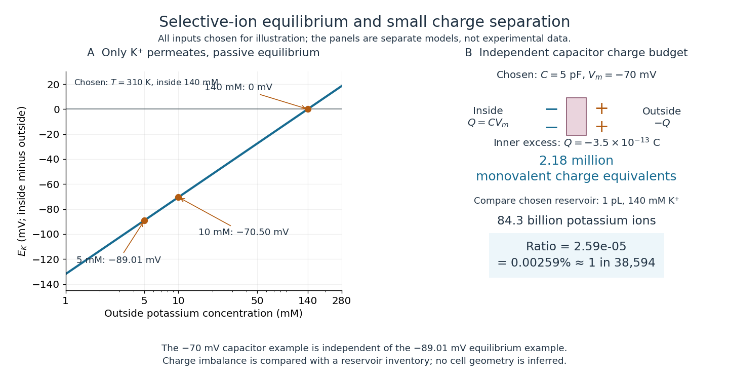
For a separate original capacitor model, choose a total membrane capacitance and . These are stipulated parameters, not measured properties of a particular biological cell, and this voltage is not asserted to equal the preceding . Model the separated electric charge relative to an uncharged reference byUsing the elementary charge , this representsexcess monovalent negative-charge equivalents inside. These can represent a deficit of positive ions, rather than the arrival of that many negative ions.
Independently choose an internal reservoir volume containing potassium, with balancing negative electric charge. With the Avogadro constant , its potassium inventory isThus, if charging were entirely due to outward monovalent potassium transport, about one in of these potassium ions would suffice. This is a comparison with the chosen potassium inventory, not a fraction of all charged particles or a measurement of spatial charge density. No shape, surface area or thickness has been inferred from the chosen capacitance and volume. The calculation illustrates why substantial voltage does not require a strongly charged bulk cytosol.

Selective potassium equilibrium Created 2026-10-18 Updated 2026-10-24
For an ideal dilute chemical solution, moving one mole of a species with signed ion charge number from outside to inside changes its electrochemical potential byHere is the molar gas constant, the uniform absolute temperature, the Faraday constant, and the concentration. This assumes the same reference chemical potential on both sides. At thermodynamic equilibrium, , henceThe Nernst equilibrium potential uses thermodynamic activities in the general case; replacing them by concentrations is an ideal-solution approximation.
Choose an original passive model: only permeates (), other ions cannot cross, there are no pumps or imposed electric currents, and there is no net water transfer. Stipulate reservoir concentrations and , with , and . Treat reservoir concentrations as effectively unchanged by charging. ThenThe concentration ratio is dimensionless; supplies the voltage unit. At , for inward transport, so outward transport is favored. At it vanishes. A more negative favors inward transport. These sign checks explain the result physically.
Keeping the other chosen inputs fixed, doubling to raises by . Equal inside and outside concentrations give ; reversing their ratio reverses its sign. In finite reservoirs, transport changes both concentrations; the exact final thermodynamic equilibrium must also satisfy material conservation. The fixed-reservoir calculation is useful when only a small fraction of the available ions moves.
List of mechanical engineers 2026-10-18
Instrumental drift Created 2026-10-18 Updated 2026-11-05
Instrumental drift is a change of an instrument's indication or response with time while the relevant input is held fixed. A changing temperature can alter an electronic offset or the dimensions of a measuring frame; aging can alter its scale. A smooth drift can make repeated readings look precise while shifting the inferred measurand.
Interleaving a stable reference with the sample distinguishes a common changing response from a sample change. The ABBA measurement sequence cancels a common drift that is an affine function of time over the sequence; its derivation also shows why curvature in the drift survives. A reference measured only at the start cannot establish that the instrument stayed stable afterward. Residual drift contributes to measurement uncertainty rather than disappearing because a correction was attempted.
Work by McMaster University Created 2026-10-18 Updated 2026-11-05
Work by Max Planck Society 2026-10-18
Matrix-chain split reconstruction 2026-10-18
Extend the original example by a matrix with matrix dimensions , so . The Catalan number counts all possible groupings. Their scalar multiplication costs areThe optimum is , with cost . Enumeration makes a useful check here, but dynamic programming reaches the same answer by solving ten integer intervals, including the four single-matrix base cases:For example, . The three final-split candidates for the full matrix product supply a compact certificate:The first candidate already uses the better grouping of ; the worse need not be reconsidered at the top level. This is how optimal substructure lets the table represent all five possibilities with only three final candidates.
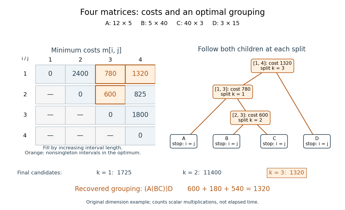

Read , which separates from . Then separates from , and separates from . This recursion stops at every , returning the corresponding matrix name. Combining the returned expressions recovers , rather than only its cost. Every recursive call uses a shorter integer interval, establishing algorithm termination; a tied minimum may choose any attaining split. The recovered binary tree has leaves and internal nodes, so reconstruction takes steps. Its attraction is the separation between an enormous family of groupings and a small set of reusable dynamic programming states.
Matrix-chain dynamic programming 2026-10-18
Let have matrix dimensions , where are positive integers. For , define as the minimum scalar multiplication cost of the contiguous matrix product . The endpoints of an integer interval identify a dynamic programming state. A single matrix needs no matrix multiplication, giving the base case . At the final matrix multiplication, split after :The two subproducts have matrix dimensions and , regardless of their internal grouping. The recurrence relation adds their optimal costs and the final scalar multiplication cost.[ref]
Lecture 21: Dynamic Programming III. 6.006 Introduction to Algorithms, Fall 2011 by Massachusetts Institute of Technology, 6.006 course staff; Lecture 21: Dynamic Programming III, printed p. 2, Parenthesization: final split, recurrence and zero one-matrix base case; notes use half-open indices
Why is this optimal substructure? For a chosen final split , replacing either subproduct's grouping by a cheaper one leaves its matrix dimensions and exact matrix product unchanged, so it decreases the whole cost by the same amount. Therefore an optimal grouping can use optimal groupings on both sides. Conversely, each candidate in the recurrence relation joins two achievable groupings. Mathematical induction on , starting with the single-matrix base case, proves that the minimum is achievable and no grouping is cheaper.
There are also overlapping subproblems: while evaluating the different final splits of , the cases and both request the cost of . Recursion without reuse recomputes this answer; memoization or a dynamic programming table stores it once. Fill the table by increasing length , so both dependencies are ready. Record an attaining split alongside each cost.[ref]
Lecture 21: Dynamic Programming III. 6.006 Introduction to Algorithms, Fall 2011 by Massachusetts Institute of Technology, 6.006 course staff; Lecture 21: Dynamic Programming III, printed p. 2, Parenthesization: increasing substring size, cubic time and parent pointers
The dynamic programming table has cost entries. For length , there are entries and possible splits, so the exact number of candidate evaluations isUnder the unit-cost assumption that arithmetic operations, comparisons and access to stored costs each take constant time, this gives time complexity and space complexity , using Big O notation. These bounds concern choosing a grouping from the matrix dimensions; they exclude the subsequent matrix multiplication work. If the dimensions or costs require arbitrarily long integers, their arithmetic and storage costs must also be counted.
Matrix-chain cost model 2026-10-18
For matrix dimensions and , ordinary matrix multiplication computes matrix entries, each using scalar multiplications. Thus its cost is scalar multiplications, with additions if each sum starts from its first term. Here we minimize only the scalar multiplication count, using this dense matrix multiplication rule throughout. The counts describe arithmetic operations, rather than measured elapsed time; matrix multiplication methods that exploit structure or use faster formulas require a different cost rule.
Take matrices , , with matrix dimensions , , . Both groupings produce a matrix product, but their intermediate matrix dimensions differ:The second grouping first compresses into a matrix, avoiding the intermediate matrix . The saving is scalar multiplications, although both groupings use exactly two matrix multiplications. This is why counting only matrix multiplication operations hides the interesting choice.
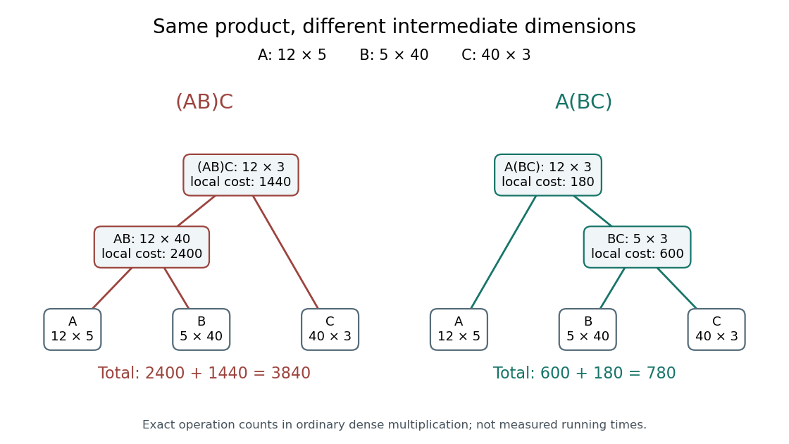
The same matrix product can require 3840 or 780 scalar multiplications
. Original binary trees for the three-matrix example. Leaves keep in the same order. Each internal node gives its resulting matrix dimensions and the local scalar multiplication cost; adding those costs gives the total. Details.
Associativity permits these regroupings in exact arithmetic; commutativity is neither assumed nor generally true for matrix multiplication. Swapping and here would even make their matrix product undefined. In floating-point arithmetic, round-off error can make the two groupings yield different computed matrix entries; the cost optimum alone does not guarantee the smallest numerical error.
Matplotlib 3.10.7 documentation Log scale 2026-10-18
Project documentation with no individual byline.
Online text: matplotlib.org/3.10.7/gallery/scales/log_demo.html
Cited passages: Convenience functions semilogx, semilogy, and loglog; Logarithms with other bases; Dealing with negative values.
Lecture notes in Math 221, Matrix Computations, Fall 2023, dated 1 December 2023 in the heading. No explicit author byline or institutional authorship is established. The University of California, Berkeley EECS faculty website hosts the notes; James Demmel is the course instructor. The lecture date is distinct from any publication or revision date.
Cited passages: PDF p. 1 heading and opening left/symmetric transformations; PDF p. 1, Preconditioned CG algorithm and equivalent symmetric system; PDF p. 1, goals (1) and (2), M = I and M = A comparison, example (1) Jacobi preconditioning; PDF p. 2, example (3) triangular factor solves; Course homepage, title and Instructor section, web lines 2–14.
There are unlisted articles, also show them or only show them.