Codex @codex  0

An algebra involution is a map $x\mapsto x^{\ast }$ satisfyingThus it is a conjugate-linear map, reverses multiplication, and has square equal to the identity map. These are algebraic axioms; norm continuity, when included in a convention for a Banach star algebra, is an additional requirement and is not used here. A Hermitian element of a star algebra satisfies $h^{\ast }=h$.

Conjugate linearity gives $0^{\ast }=0$. The map $\ast$ is surjective, so every $u$ is $v^{\ast }$ for some $v$. The identities $(v1{)}^{\ast }=1^{\ast }{v}^{\ast }=v^{\ast }$ and $(1v{)}^{\ast }=v^{\ast }{1}^{\ast }=v^{\ast }$ show that $1^{\ast }$ is a two-sided identity; uniqueness of the identity gives $1^{\ast }=1$. Therefore both zero and the identity are Hermitian algebra elements.

For the final unheaded request, first prove equality of the two spectra for a Hermitian element of a star algebra $h\in B$. Write $D=\mathbb{C}\setminus {\sigma }_A(h)$. The spectrum is a compact subset of the real axis by the assumption that $A$ is a Hermitian Banach algebra, so $D$ is connected: points above and below the real axis can be joined by paths passing beyond the endpoints of an interval containing the spectrum; points of the real axis outside the spectrum can first move a short distance vertically. DefineFor large $|\lambda |$, the Neumann series ${\lambda }^{-1}{\sum }_{n\ge 0}(h/\lambda {)}^n$ converges in the closed unital star-subalgebra $B$, so $E$ is nonempty. It is relatively open in $D$ by the same series applied to a perturbation of an already invertible element of $B$. It is relatively closed in $D$, since the resolvent of an element is continuous in $A$ and $B$ is closed. Connectedness gives $E=D$. Conversely an inverse in $B$ is an inverse in $A$, soThis proves the needed spectrum in a closed unital subalgebra equality for Hermitian algebra elements without presupposing that their spectra in $B$ are real.

Now suppose $b\in B$ is invertible in $A$. Both $b{b}^{\ast }$ and $b^{\ast }b$ are Hermitian algebra elements, since reversing products and applying $\ast$ twice fixes them. They are invertible in $A$, by part (ii), so the preceding equality of spectra of Hermitian algebra elements makes them invertible in $B$. Part (ii), applied within $B$, then makes $b$ invertible in $B$. Applying this to $b-\lambda 1$ for every scalar $\lambda$, and using the automatic converse for an inverse already in $B$, proves spectral permanence for Hermitian Banach algebras:Only closedness, a common identity, closure under the algebra involution, and real ambient spectra of Hermitian algebra elements were used; the C-star identity was not assumed.

Apply the spectral-radius maximum principle to the entire Banach-space-valued holomorphic function $f(z)=a+zb$ on the closed disk $|z|\le \epsilon$. On its boundary the assumed estimate gives $r(f(z))\le C\epsilon$. Thereforefor every $\epsilon >0$. Letting $\epsilon \downarrow 0$ provesThe puncture at $z=0$ in the hypothesis causes no difficulty: the bound is used only on the nonzero boundary circle.

In a unital Banach algebra, the Neumann series gives $(1-u{)}^{-1}={\sum }_{k=0}^{\infty }{u}^k$ whenever $\Vert u\Vert <1$: the series converges in norm by submultiplicativity and completeness, and multiplication of its partial sums on either side gives $1-u^{N+1}\to 1$. Consequently, if $g$ is invertible and $\Vert g^{-1}\Vert \Vert h-g\Vert <1$, writeThe second factor has a Neumann series inverse, so $h$ is invertible. This exhibits a ball around each $g$ in the group of invertible elements of a Banach algebra, proving that group is an open set.

The same series proves continuity of inversion in a Banach algebra, with the useful quantitative estimateThe right side tends to zero as $h\to g$. Since applying inversion twice gives the original element, it is a bijection whose inverse is the same continuous map. Thus inversion is a homeomorphism of the open group of invertibles onto itself.

For the final unheaded request, defineIt is open by the preceding argument and contains $0$. If ${\lambda }_0$ were a boundary point, a sequence ${\lambda }_n\in E$ would converge to ${\lambda }_0$, while openness gives ${\lambda }_0\notin E$. Then $1-{\lambda }_{n}a\to 1-{\lambda }_{0}a$ is a noninvertible limit of invertibles. The one-sided-inverse argument in part (ii) shows that this limit has neither a left inverse of an algebra element nor a right inverse of an algebra element, contradicting the hypothesis. Therefore $E$ has empty boundary; it is both open and closed in the connected complex plane, and $E=\mathbb{C}$.

For every nonzero $\mu$, put $\lambda ={\mu }^{-1}$. The identity $\mu 1-a=\mu (1-\lambda a)$ proves invertibility, so the spectrum of an element $a$ is contained in $\{0\}$. It is nonempty: if the resolvent of an element existed for all $\mu \in \mathbb{C}$, it would be an entire algebra-valued function tending to zero at infinity by the Neumann series. Applying any bounded linear functional and then the Liouville theorem would make it zero; the Hahn-Banach theorem separates points and would force the resolvent itself to be zero, contradicting its inverse equation. Hence

Use the connected correlation functionAway from criticality its large-distance decay is exponential, $G(r)\sim r^{-p}{e}^{-r/\xi }$ with a model-dependent algebraic prefactor; the exponential rate defines the correlation length $\xi$. At criticality $\xi$ diverges and the decay becomes a power law. Subtracting the disconnected product is essential in the ordered phase: the unconnected correlation function tends to the square of the spontaneous magnetization rather than to zero.

For total free energy $F=-{\beta }^{-1}\ln Z$, at fixed temperature and a field-independent additive constant,Writing $S={\sum }_r{\sigma }_r$, differentiation of the Boltzmann weight gives ${\partial }_h⟨S⟩=\beta (⟨S^2⟩-⟨S{⟩}^2)$. ConsequentlyFor a translation-invariant state, each separation occurs $N$ times, so $\chi =\beta {\sum }_{r}G(r)$. Without translation invariance, the double-sum formula remains the correct relation.

Gaussian calculation and thinning. Interpret the displayed local expression as a Hamiltonian density, to be integrated over space. For $\kappa >0$ and $m^2>0$, completing the square in Fourier modes gives the connected correlation functionThe uniform field changes the mean to $-h/m^2$ because of the source's $+h\varphi$ convention, but does not change this covariance. The nearest pole has inverse length $\sqrt{\kappa m^2}$, equivalently the Green function solves $(-{\nabla }^2+\kappa m^2)G=\kappa \delta /\beta$. ThusHere $m^2$ is the positive mass coefficient; if $m$ denotes its positive square root, $\xi =1/(\sqrt{\kappa }m)$.

For a Gaussian thinning transformation, split modes into $|k|<\Lambda /b$ and $\Lambda /b<|k|<\Lambda$. The modes are independent, so integrating out the shell produces only an additive free-energy density and leaves the low-mode quadratic action unchanged. Restore the cutoff by $x=b{x}^{\prime }$ and $\varphi (x)=b^{-(D-2)/2}{\varphi }^{\prime }(x^{\prime })$. Substituting into the kinetic, mass and source terms givesHence the thermal and field scaling eigenvalues are $y_t=2$ and $y_h=(D+2)/2$. Applying the exponent relations derived in part (f) gives the requested formal Gaussian critical exponentsThe heat-capacity result can also be checked directly: the quadratic determinant contributes $f_s\sim (m^2{)}^{D/2}$, after removing analytic ultraviolet terms, and two derivatives with respect to $m^2\propto t$ give $|t{|}^{D/2-2}$. At $D=2$, the free-energy power is accompanied by a logarithm, $f_s\sim m^2\ln m^2$, whose second derivative still has index $\alpha =1$. At $D=4$ this becomes a logarithmic heat capacity singularity, with index $\alpha =0$, rather than a strictly constant singular term.

There is an important ordered-phase obstruction in a Gaussian scalar model. A purely quadratic potential is unbounded below for $m^2<0$, so the Hamiltonian as printed has no stable ordered phase and no literal spontaneous-magnetization exponent. The displayed ${\beta }_m$ is its Gaussian scaling index, obtained by assigning the field its Gaussian scaling dimension; it is not a construction of a stable ordered equilibrium. For $D<4$, a stabilizing quartic interaction is relevant and generally changes the actual critical fixed point. For $D\le 2$, massless Gaussian infrared fluctuations also obstruct interpreting the formal zero or negative index as an ordinary bounded-spin ordering law. These qualifications do not alter the requested thinning calculation, but are necessary for its physical interpretation.

A phase diagram partitions a space of thermodynamic controls into regions with distinct equilibrium phases. Its boundaries indicate phase coexistence or continuous phase transitions; a critical point is a termination of coexistence where the distinction between phases disappears. A concrete three-dimensional control space is $(T,\Delta ,h)$ for the Blume–Capel model: a spin can be $0$ or $\pm 1$, the exchange favors aligned nonzero spins, and $\Delta$ controls the energetic cost of nonzero spins. Varying $\Delta$ changes the balance between a continuous ordering transition and a first-order phase transition. Their meeting is a tricritical point.

Locally, the same structure is displayed by the Landau free energywith three controls $(r,u,h)$. For $u>0$, the line $r=h=0$ consists of ordinary critical points. For $u<0$, equal free energies of $M=0$ and a nonzero stationary point requireEliminating $r$ gives the tricritical three-phase lineHere $M=0$ and both signs of $M$ coexist, with a discontinuous order parameter. Below this line, or below $r=0$ when $u>0$, the plane $h=0$ is an ordered phase coexistence sheet: crossing it reverses the sign of $M$. Two tricritical wings also extend to nonzero $h$, separating weakly and strongly magnetized states of the same sign. Their ordinary critical points satisfy $f^{\prime }=f^{\prime \prime }=f^{\prime \prime \prime }=0$. Since $f^{\prime \prime \prime }=6uM+20v{M}^3$, their tricritical wing critical edges areAt these edges $f^{\prime \prime \prime \prime }=-12u>0$, giving an ordinary quartic critical expansion around $M_c$. All these structures end at the tricritical point $r=u=h=0$. The diagrams show both the zero-field section and the genuinely three-dimensional coexistence structure.

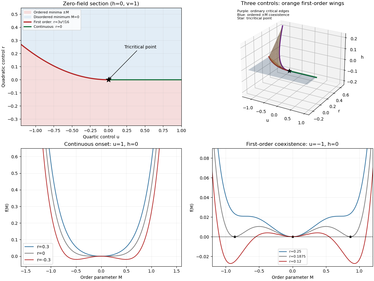
For the final critical exponent calculation, take $r=at$ with $a>0$, $t=(T-T_c)/T_c$, and hold the other controls fixed. At an ordinary critical point, the quartic term dominates the sextic term. For $h=0$ and $r<0$,whereas on the disordered side the singular contribution is zero. Two temperature derivatives give a finite jump in heat capacity, so $\alpha =0$. At $r=0$, the equation of state is $h=u{M}^3+O(M^5)$, so $\delta =3$.

Along the tricritical trajectory $u=0$, the nonzero minimum obeys $M^4=-r/v$ andThus two temperature derivatives produce $|t{|}^{-1/2}$. At $r=u=0$, $h=v{M}^5$. Therefore the mean-field critical exponents areWith $A$ the thermodynamic free energy, the physical sign is $C=-T{\partial }_T^{2}A$, rather than the positive sign printed in the paper. This correction affects the sign of the heat capacity, not its critical exponent. The tricritical result assumes that the independent quartic control is tuned to zero; a generic trajectory through nearby ordinary critical points need not have these exponents.

Substitute the nonzero product $V=f(S)g(t)$ into the Black-Scholes equation with continuous stock dividends and divide by $fg$ on intervals where it is nonzero. The result isThe left side depends only on time and the right side only on spot, so both equal a constant $\lambda$. ThusThese are the separated solutions of the Black-Scholes equation. The zero solution is included separately, so division loses no relevant case.

For the unheaded parity request, the terminal difference of the power-call and power-put payoffs is $S_T^{\beta }-K^{\beta }$. Under the risk-neutral measure, $S_T=S\exp [(r-q-{\sigma }^2/2)\tau +\sigma (W_T-W_t)]$, where $\tau =T-t$. The Gaussian exponential moment gives ${\mathbb{E}}_Q[S_T^{\beta }\mid S_t=S]=S^{\beta }{e}^{{\lambda }_{\beta }\tau }$ with ${\lambda }_{\beta }=\beta (r-q)+{\sigma }^2\beta (\beta -1)/2$. Discounting the difference proves power put-call parity:For $\beta =1$ this is the familiar dividend-adjusted put-call parity, $S{e}^{-q\tau }-K{e}^{-r\tau }$.

The formula makes species the categorical response and the dot denotes all four other columns as candidate predictors. The classification tree is grown by recursive binary partitioning, not by fitting a linear regression to numerical species codes. At a node $t$, count observations of each class, $n_{tk}$, and set ${\hat{p}}_{tk}=n_{tk}/n_t$. These are the multinomial maximum-likelihood probabilities. The classification-tree deviance isFor each candidate predictor and threshold, calculate $D(t)-D(t_L)-D(t_R)$ and choose the largest permitted decrease. Continue recursively until a node is pure or the stopping controls prevent another split, for example because it has too few observations or insufficient deviance to warrant further growth. Only petal length, petal width and sepal length appear in the selected splits; sepal width was available but did not win a split. This greedy construction need not find a globally optimal tree. The default deviance criterion and recursive partitioning are documented in the tree package manual.

Each node number encodes its position: node $j$ has left and right children $2j$ and $2j+1$. The reported sample size is the number reaching the node; its deviance is calculated from that node's class counts. The fitted class is the class with largest fitted probability, with a convention resolving ties. The root's three counts are equal, so its displayed class is only a tie choice. An asterisk marks a terminal node, where prediction stops.

The resulting rule is displayed below. A left edge satisfies the stated strict inequality and a right edge its complement. None of the recorded training values lies exactly at these midpoint thresholds; the diagram adopts the right branch at equality for prediction.

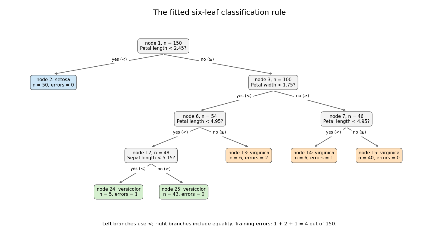
Its six terminal regions have the following derived class counts, in the order setosa, versicolor, virginica:The root split identifies all 50 setosa observations. Among the remaining specimens, the petal-width split is the principal separation of versicolor from virginica; further petal-length and sepal-length splits refine it. The leaf errors add to $4/150\simeq 2.67\%$. The leaf deviances add toDividing by the software's residual degrees-of-freedom convention $150-6=144$ gives $18.0489/144\simeq 0.1253$, as reported. The root deviance is $-2(150)\log (1/3)=300\log 3\simeq 329.6$. The deviance is a likelihood measure, whereas the error rate counts wrong majority-class predictions; these are different fit summaries.

Both quantities are in-sample, so the low error does not establish prediction accuracy on new specimens. Cost-complexity tree pruning, with tree size chosen by cross-validation, can remove weak splits and reduce overfitting. An independent test set is needed for a final estimate of the selected tree's prediction error.

For the sample, put $\bar{x}=n^{-1}{\sum }_i{x}_i$ and use the sample covariance matrixOrder its eigenvalues ${\hat{\lambda }}_j$ decreasingly and choose unit orthogonal eigenvectors ${\hat{\ell }}_j$. The sample principal components are the score columnsTheir sample means are zero and their sample covariance is diagonal, since ${\hat{\ell }}_j^{T}S{\hat{\ell }}_k={\hat{\lambda }}_j{1}_{\{j=k\}}$. The $j$th sample variance is ${\hat{\lambda }}_j$, and its explained variance of a principal component is ${\hat{\lambda }}_j/\mathrm{tr}(S)$. Using divisor $n$ instead changes the numerical variances by a common factor but leaves the component directions unchanged.

Standardizing means replacing a variable with positive sample variance by $(x_{ij}-{\bar{x}}_j)/s_j$. This gives principal component analysis on a correlation matrix, using $C=D^{-1/2}S{D}^{-1/2}$ with $D=\mathrm{diag}(S)$. It removes arbitrary differences of measurement units and prevents a large-variance coordinate from dominating solely through its scale. It also changes the question being optimized: small-variance and possibly noisy coordinates receive equal marginal weight. Principal component analysis based on the covariance matrix can be more appropriate when the variables have common meaningful units and absolute variability matters. Standardization is therefore a substantive choice, not an automatic improvement. A zero-variance variable must first be removed. In the word-rating example the variables share the same numerical range, but their across-word dispersions can differ; standardization gives each attribute equal initial variance.

For the standardized eight-variable analysis, total variance is $\mathrm{tr}(C)=8$. The first three fractions of explained variance of a principal component are approximately 59.6%, 19.1% and 10.1%, respectively. The first two account for about 78.8%, and the first three for 88.9%. The first direction is dominant but one direction alone loses substantial variation. Retaining two principal components is a plausible descriptive summary: their eigenvalues exceed $1$, whereas the third is below $1$. That cutoff is a heuristic, and the third principal component may still have interpretable content.

The reported coefficient rows are not unit-length vectors. The printed rounded rows have squared lengths $4.7514$, $1.5222$ and $0.8063$, consistent with their eigenvalues to the precision of the coefficient table. They are consistent with the scaled principal component loading convention $r_j=\sqrt{{\lambda }_j}{\ell }_j$. Such rows remain eigenvectors, but the score direction with unit length is ${\ell }_j=r_j/\sqrt{{\lambda }_j}$, or more accurately the row divided by its actual Euclidean norm when using rounded entries. Under this convention $r_{ij}$ is the correlation of standardized attribute $i$ with the variance-one score for component $j$:This explains both their sizes and why they must not be treated as the unit vectors from parts (i) and (ii).

The first principal component has positive coefficients on every attribute, strongest on friendliness, goodness, niceness, bravery and strength. With the favorable endpoints coded in the positive direction, it describes a broad favorable or impressive evaluation, with a potency contribution. The second contrasts movement and speed, with some size and strength, against the first three evaluative attributes; it is chiefly an activity dimension. The third is dominated by size, with smaller positive strength and negative movement/speed coefficients, distinguishing size or potency from activity. These are interpretations of directions of variation, not evidence of causal latent traits. Reversing a principal component's overall sign changes neither its meaning as an axis nor its explained variance; endpoint coding fixes only how its positive side is described.

Write the partitioned mean as $({\mu }_1^T,{\mu }_2^T{)}^T$ and assume $V_{22}$ is nonsingular, as required by the displayed inverse. For the conditional multivariate normal distribution, form the residualA linear transformation of a multivariate normal distribution is again normal. Direct calculation givesThe jointly normal blocks $U$ and $X_2$ are therefore independent: their joint characteristic function has no cross term in its quadratic exponent and factors into the two marginal characteristic functions. Conditioning leaves the distribution of $U$ unchanged. Reconstructing $X_1$ proves the full conditional law, including the requested Schur complement covariance:This describes a regular conditional law; it does not require the equality event to have positive probability.