
Perfect quantum error-correcting code 2026-10-14
A nondegenerate quantum code is perfect at correction radius if its distinct correctable Pauli error images exhaust the physical Hilbert space. Each image has dimension , and their orthogonal direct sum is the whole -dimensional space precisely when the quantum Hamming bound is an equality. This perfectness concerns unknown-location errors of weight at most ; it does not imply correction of every higher-weight error.
Quantum integer Created 2026-10-14 Updated 2026-11-05
The symmetric quantum integer is the displayed Laurent polynomial, with . It obeys and . At a primitive odd th root of unity, exactly when divides .
Highest-weight string for quantum sl2 2026-10-14
If and , induction using the defining commutator gives the displayed identity. When is not a root of unity, a finite string of length in a simple module has , . Its distinct eigenvalues make the string vectors independent, and the nonzero raising coefficients prove simplicity.
Cubic-root quantum-plane socle 2026-10-14
At a primitive cube root of unity, the cubic homogeneous module has basis . Its only simple modules occurring as submodules are the one-dimensional subspaces of , on which and . Its quotient by this two-dimensional submodule is simple, but it has no simple complement: any lift of the highest weight space contains , whose image is . Thus the cubic module is not a semisimple module.
One-loop scalar effective potential 2026-10-14
For one canonically normalized real scalar field and , the modified minimal subtraction scheme gives the displayed one-loop term. The Gaussian fluctuation approximation produces . Its derivative in is half the Euclidean massive loop integral with . Integrating and subtracting its pole yields the formula, up to a field-independent constant. Other finite counterterms alter the scheme-dependent nonlogarithmic part. Negative curvature requires an analytic continuation and can yield an imaginary part indicating instability of that background.
For a bipartite pure state with finite Von Neumann entropy, the joint Von Neumann entropy is zero, so its quantum conditional entropy is . The Schmidt decomposition makes the nonzero eigenvalues of the squared Schmidt coefficients. Their Shannon entropy vanishes exactly when there is one coefficient, equivalently the joint pure state is a product state. Thus negative quantum conditional entropy detects exactly the entangled bipartite pure states; it is only a sufficient criterion for entanglement of general mixed density operators.
Quantile endpoint at probability one Created 2026-10-14 Updated 2026-11-05
The quantile function is finite at every probability strictly between zero and one, but need not be finite at one. For any unbounded-above normal distribution, for every real , so its generalized inverse at one is . Inverse transform sampling still produces a real random variable almost surely because a continuous uniform distribution puts zero mass at that endpoint. A real-valued implementation may discard endpoint draws or assign an arbitrary finite value there without changing the sampled law.
Sample quantile Created 2026-10-14 Updated 2026-11-05
For observations and , the sample quantile in the generalized-inverse convention iswhere is the empirical distribution function and the observations are ordered with ties retained. For five observations, the sample median in this convention is the third order statistic. Interpolated sample-quantile conventions can give different finite-sample answers.
For the asymptotic statement, assume the observations are independent and identically distributed with cumulative distribution function . Let be its unique -quantile, and suppose has a density continuous and strictly positive at . ThenFor a proof, is exactly the event that at least observations are at most . At , the count is binomial with success probability . The binomial central limit theorem gives the displayed normal limit. A larger density at the target quantile makes the quantile more precisely estimated. The independence and local-density hypotheses are needed; the formula cannot be applied unchanged to arbitrary dependent observations or an atom.
Probable error Created 2026-10-14 Updated 2026-11-05
The probable error is the half-width of an interval around a specified central value containing probability . For a normal distribution with , its quantile function giveswhere is the standard normal cumulative distribution function and is the standard deviation. The factor is specific to the normal distribution. The centered Cauchy distribution with parameter has probable error , despite having no finite variance. Thus a central probability width need not require a finite second moment.
Far-zone quadrupole strain 2026-10-14
In units , a slowly moving isolated source has trace-free mass quadrupole moment . The retarded linearized gravity solution and the stress-energy quadrupole identity give the displayed physical spatial strain, with and the transverse-traceless projector . If the spatial metric is written for metric signature , its trace-free Lorenz-gauge coefficient before the transverse projection is . Thus . Far distance alone does not permit dropping source-dependent retardation: the quadrupole approximation also requires the source size to be small compared with the radiation wavelength.
Bretschneider's formula 2026-10-14
For a quadrilateral with side lengths , semiperimeter , area , and opposite angles ,The second term vanishes exactly when , which is the cyclicity condition for a nondegenerate convex quadrilateral.
Parallelogram 2026-10-14
A parallelogram is the convex set with vertices for two linearly independent planar vectors . Its opposite edges are parallel and its centre gives central symmetry. Its area is , so an invertible linear map changes its area by the absolute value of that map's determinant. These facts make parallelograms convenient convex bodies for two-dimensional applications of the Minkowski convex body theorem.
Rectangle Created 2026-10-14 Updated 2026-10-20
Simpson's rule Created 2026-10-14 Updated 2026-10-18
Simpson's rule approximates a definite integral by integrating the quadratic polynomial obtained by polynomial interpolation at two endpoints and their midpoint. For an interval with , write and . The three quadrature nodes are , and the quadrature rule isThus its quadrature weights are . Their sum is , as required for exactness on constant functions. This is the three-node Newton-Cotes closed quadrature; its degree of precision of a quadrature rule is three, even though the interpolating polynomial has polynomial degree at most two.[ref]
3.5 Quadrature, subsection (ii) Simpson’s Rule. NIST Digital Library of Mathematical Functions; §3.5(ii), equation 3.5.6: elementary Simpson rule and its fourth-derivative remainder
For an original worked example, take the cubic polynomial on the interval . Here and , so the function evaluations giveSimpson's rule givesAn antiderivative supplies an independent exact definite integral:The quadratic polynomial through the same quadrature nodes is . It differs from between the quadrature nodes, but its definite integral agrees exactly. The picture shows why: the signed polynomial interpolation error has two lobes with opposite integrals.
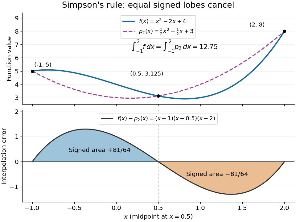
An original cubic and its quadratic interpolant have the same integral because the two interpolation-error lobes have signed integrals plus and minus 81 over 64
. Details. 
Three function evaluations therefore capture more information about an integral than about the whole function. When an antiderivative is unavailable, composite Simpson's rule repeats this inexpensive local construction over a partition of an interval. For a sufficiently smooth function, halving the node spacing reduces its truncation error by approximately a factor of sixteen.
Newton-Cotes closed quadrature 2026-10-14
Integrate the Lagrange polynomial through values at all equally spaced nodes , including both endpoints. The resulting quadrature rule is exact through degree . For even , the node polynomial is odd about , so its integral vanishes and exactness extends through degree . The weights need not remain positive as the number of nodes increases.
Noise sensitivity of a quadrature rule 2026-10-14
If the observed samples are , the resulting quadrature rule changes by . Bounded sample perturbations therefore satisfyFor ordinary numerical integration with nonnegative quadrature weights exact on constant functions, the bound is , independent of panel refinement. A common bias attains it: the quadrature error due to the function approximation may vanish while this sample error persists. Interpolating a fixed data set onto a finer grid likewise does not create new observations or remove its uncertainty.
With new samples whose errors are independent random variables of zero expectation and common variance , a different model givesFor equal panels this is for the composite midpoint quadrature rule and for the composite trapezoidal rule. These variance reductions require the stated independence and unbiasedness assumptions; a common bias or correlated sample errors need not shrink. The two displayed perturbation formulas follow directly from the triangle inequality and the variance additivity for independent random variables, respectively.
Degree of precision of a quadrature rule 2026-10-14
The degree of precision of a quadrature rule is the largest integer such that for every polynomial of polynomial degree at most . By linearity, checking the monomials suffices. Exactness for one higher-degree polynomial alone does not raise this degree: every lower polynomial degree must also be covered.
Quadrature weight 2026-10-14
A quadrature weight multiplies a sampled integrand value in a quadrature rule. For ordinary numerical integration, its units match those of the integration variable. Positive quadrature weights that sum to make a weighted average of the samples; signed quadrature weights can magnify sample perturbations, as quantified by noise sensitivity of a quadrature rule.
Quadrature node Created 2026-10-14 Updated 2026-10-31
A quadrature node is a point at which the integrand is sampled by a quadrature rule. Under the affine map from to , a reference quadrature node becomes ; for ordinary numerical integration, the corresponding quadrature weight is multiplied by .
Quadratic-inflation endpoint estimate 2026-10-14
For and unreduced Planck mass , the potential slow-roll parameter is . Its conventional value one gives the displayed endpoint estimate. Exact accelerated expansion ends at , or for a canonical scalar alone. Substitution of slow-roll formulas into this exact condition gives a different order-one coefficient because slow roll is failing there; a precise endpoint requires integrating the full inflaton equation of motion and Friedmann equation. The large-field e-fold estimate is insensitive to this order-one endpoint uncertainty.
There are unlisted articles, also show them or only show them.