
Power-law initial-mass-function tail coordinate Created 2026-10-14 Updated 2026-11-05
For an initial mass function proportional to on with , integration and normalization give the displayed upper-tail fraction. The probability integral transform makes uniform on for a randomly sampled birth mass. Evolutionary lifetime regions can then be measured as ordinary areas when the independent age coordinate is also uniform.
If a cohort is periodically confirmed event-free but exact event reports update only those who fail, censoring the remaining subjects at their last scheduled confirmation creates informative censoring. Between confirmations the nominal risk set retains future observed failures and removes nonfailures. An apparent final failure may therefore empty the recorded risk set even though other cohort members remain event-free. Use a common verified cutoff or a complete event register with a common administrative censoring date.
Sensitivity curve Created 2026-10-14 Updated 2026-11-05
Add one observation to the empirical sample, so . The displayed finite difference is a finite-sample counterpart of the influence function. Its supremum magnitude measures worst-case one-observation sensitivity; unlike an infinitesimal derivative it records the actual response at contamination fraction .
Empirical influence function Created 2026-10-14 Updated 2026-11-05
This plugs the empirical distribution into the population influence function. For an M-estimator it is , when this denominator is well-defined and nonzero. For functionals involving a density at a quantile, an unsmoothed empirical measure may not permit this derivative, so smoothing or an actual sensitivity curve is required.
Influence function of a quantile Created 2026-10-14 Updated 2026-11-05
Let be the unique th quantile, with , and suppose the density is continuous and positive at . Define quantiles of contaminated distributions using the generalized inverse. For , differentiating givesAt , the generalized-inverse quantile stays exactly under this contamination, so its derivative is zero. The step formula thus holds -almost everywhere and determines the asymptotic variance . Its gross-error sensitivity is , but its local-shift sensitivity is infinite because of the jump.
Local-shift sensitivity Created 2026-10-14 Updated 2026-11-05
The local-shift sensitivity of a scalar statistical functional isIt measures the sensitivity of the first-order contamination effect to moving the contaminating observation. If the influence function is continuously differentiable with bounded derivative, the mean value theorem gives , and taking proves equality. A jump in the influence function makes infinite, even when gross-error sensitivity is finite.
Rejection point of an influence function 2026-10-14
For observations expressed in centered, standardized coordinates, the rejection point iswith value if the set is empty. A finite rejection point means sufficiently distant contamination has zero first-order effect. Boundedness of the influence function does not imply a finite rejection point: the influence function of a quantile has nonzero constant tails. Nor does tending to zero at infinity guarantee a finite rejection point unless those tails become identically zero.
Local influence versus replacement breakdown 2026-10-14
The influence function describes an infinitesimal change at a specified reference probability distribution. The replacement breakdown point asks how many observations in a particular finite sample can be replaced before an estimator becomes unbounded. The finite-sample maximum bias records the intervening changes. These are different questions: a bounded influence function at one baseline is not a general bound over all epsilon-contamination neighborhoods, nor a proof of a positive replacement breakdown point.[ref]
The Influence Curve and Its Role in Robust Estimation by Frank R. Hampel. Frank R. Hampel, The Influence Curve and Its Role in Robust Estimation, §4, p. 386: exact asymptotic curve supplemented by behavior at other distributions, especially empirical ones
The mean illustrates agreement between local and global fragility: its gross-error sensitivity is infinite and one replacement can send the sample mean arbitrarily far. The median has finite gross-error sensitivity under the stated positive-density assumptions, while its sample median withstands fewer than about half the observations being replaced under ordinary tie conventions. Its population contamination bias above still diverges as when the atom remains beyond the shifted median. Here must also move outward; taking that limit with a fixed finite atom would invalidate the displayed quantile formula.
For scalar location with a fixed positive scale, the Huber score has a direct global argument: if strictly more than half of the sample stays fixed, then beyond every retained observation by more than , their saturated scores outweigh all possible replaced scores. Every root therefore stays in a bounded interval. This is a separate finite-replacement argument; estimating scale changes its premises. A smooth bounded influence function is valuable local protection, but global robustness also depends on the full estimating rule, scale choice, and root selection.
Finite contamination bias of normal location 2026-10-14
Consider the population statistical model . The following are deterministic statistical functional calculations, not observed contamination experiments. Compare the actual location bias with the linear approximation . The mean bias is exactly . For positive exceeding the shifted median and , the generalized-inverse median bias is exactlyThis formula applies to both and throughout the plotted interval . If the contaminating atom lies inside the quantile jump containing probability , the generalized-inverse median instead equals that atom.
For the Huber location estimator with and , solve its actual population equation, rather than substituting the influence function:Writing and , integration of the normal distribution giveswhere is the probability density function of . Its derivative is , so the mixture score is strictly decreasing for . For , its limits at negative and positive infinity have opposite signs even with arbitrary distant point contamination. The displayed examples use the unique root, evaluated by the bisection method to numerical precision.
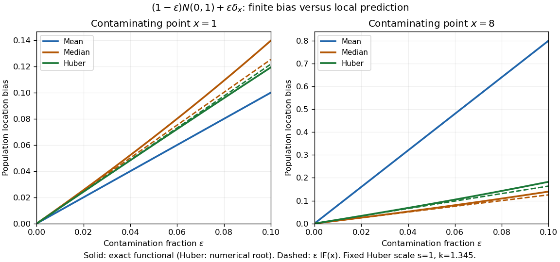
Exact population contamination biases and first-order influence predictions for normal location at contaminating points 1 and 8
. Details. At and , the exact mean, median, and Huber location estimator biases are , , and ; the influence function predictions are , , and . At , they become , , and , versus predictions , , and . The bounded alternatives control the effect of the distant atom, but their actual response curves bend away from the tangent.
The nearby atom gives a useful comparison: at , the Huber location estimator bias is , slightly below its linear approximation , whereas the median bias is still . The direction and size of approximation error depend on the contaminating location. Even accurate local influence calculations must specify , the scale, the cutoff, and the actual contamination fraction.
Normal-location influence curves 2026-10-14
For , put . The influence function of the mean, influence function of the sample median, and influence function of a Huber location estimator with fixed are respectivelyThe first grows without bound, the second jumps at the median, and the third clips continuously. For , and the normalized Huber tail is about . This illustrates the optimal bounded influence function for normal location without asserting that this cutoff is optimal for every contamination model.
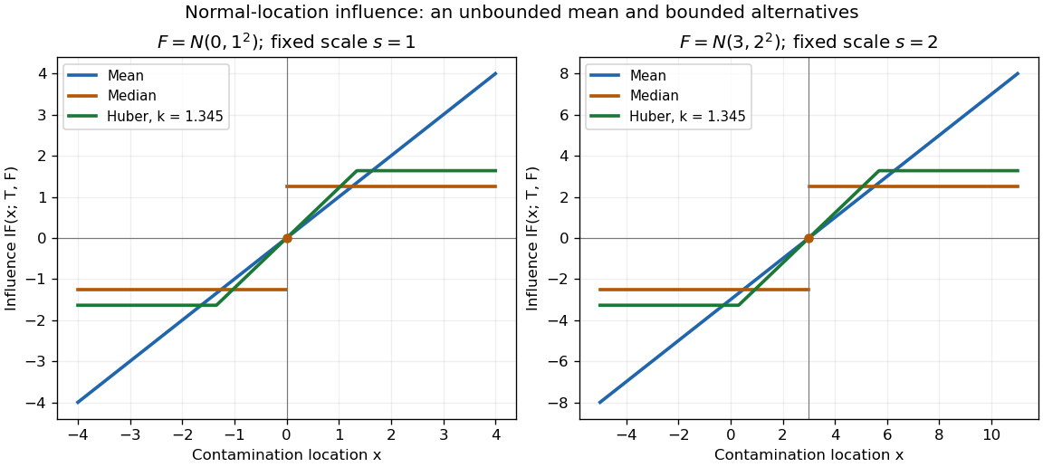


Both panels are theoretical normal distributions, with no sampled or observed data. Doubling doubles the vertical influence function scale and the horizontal clipping distance. Changing translates the curves. The isolated dot marks the actual median derivative at the center; connecting its two tails by a vertical segment would misrepresent that value. Bounded influence does not mean every small residual has less effect than on the mean: the central Huber slope is , a price paid for reducing sensitivity in the tails.
Fix a scale and cutoff . Define the population Huber location estimator by the rootHere is the Huber score. It has Lipschitz continuity, so dominated convergence justifies differentiation when puts no mass at . Then , and the nonzero derivative identifies the local population root. The implicit function theorem applies away from the contaminating score's kinks; its Lipschitz continuity also gives the first-order expansion at those kinks. Differentiating its contaminated equation yieldsThe normalization matters: the Huber score alone is not the influence function. The gross-error sensitivity is , while the rejection point of an influence function is infinite because the clipped tails stay nonzero. The original clipped estimating criterion and its derivative normalization also appear in the population analysis of M-estimators.[ref]
Robust Estimation of a Location Parameter by Peter J. Huber. Peter J. Huber, Robust Estimation of a Location Parameter, §3, p. 78: derivative normalization; §4(iii), p. 79: clipped location criterion and central-mass denominator
Scale sets what counts as a large residual. For a normal distribution with fixed , symmetry gives and , where is the standard normal distribution function. If the scale is instead a statistical functional , differentiation of the joint equation adds the scale contribution:Under a symmetric baseline and an odd Huber score, , so scale estimation drops out at first order. This cancellation needs regularity of and does not protect finite contamination changes: an inflated standard deviation enlarges the physical cutoff . A robust choice, such as a suitable Scale M-estimator, needs its own influence function and breakdown point checked. Fixing a numeric cutoff in raw units also sacrifices scale equivariance when units change.[ref]
Robust Estimation of a Location Parameter by Peter J. Huber. Peter J. Huber, Robust Estimation of a Location Parameter, §11, pp. 95-96: estimating location when normal-component scale and contamination fraction are unknown
Influence function of the mean 2026-10-14
For the statistical functional , assuming , the contaminated mean is exactlyThus the influence function of the mean is , and its gross-error sensitivity is infinite on an unbounded sample space. The linear approximation is exact here: any fixed positive contamination fraction allows an arbitrarily large change by moving far enough. No finite second moment is needed for this derivative, although a finite variance is needed for the usual central limit theorem for the sample mean.
For comparison, the influence function of the sample median iswhen the median is unique and the probability density function is positive and continuous at . The sign function records which side of receives the contaminating mass. The influence function of a quantile supplies the short derivation. With the generalized-inverse quantile convention, contamination exactly at leaves the median at , giving derivative zero there. If is very small, this bounded influence function can still be large; if , the displayed formula is unavailable.
Dynkin's formula Created 2026-10-14 Updated 2026-11-05
For a Markov process with infinitesimal generator and a suitable test function , the displayed process is a local martingale. With integrability it is a true martingale and yields the corresponding expectation identity at admissible stopping times. For bounded in the semigroup generator domain, . The Markov property applies this identity conditionally over each interval, proving the martingale increments have zero conditional expectation. Localization gives the local version. For a continuous diffusion, these identities are the martingale problem for .
Semigroup commutation with its unbounded generator Created 2026-10-14 Updated 2026-10-25
For a strongly continuous semigroup, apply the bounded operator to the difference quotient defining its semigroup generator. The limit proves domain invariance and commutation on the generator domain. This is not an assertion that the unbounded generator acts on every vector.
// Target: analysis.bigb
Tarski monster group Created 2026-10-14 Updated 2026-11-05
Buchi game 2026-10-14
In a turn-based game on a set of positions, Player I wins if the play visits a specified set infinitely often. Such games are determined even on infinite arenas. With meaning positions where I can force the next position into , the winning region is the greatest fixed point of . Inner ordinal ranks force the next visit; outer removal ranks give Player II only finitely many visits outside the winning region.
Covering of an infinite game 2026-10-14
A covering consists of a new game tree, a length-preserving prefix map to the original tree, and maps taking strategies of each player to strategies of that same player. Every play following a projected strategy lifts to a play following the original strategy, with identical projection or a premature terminal loss for that strategy's player. Terminal outcomes inherited from the original tree are respected. The strategy maps are local in depth. These conditions transfer every winning strategy, for any payoff pulled back by the prefix map. A -covering leaves all positions, outcomes and strategy choices through depth unchanged.
Approximation property of an infimum 2026-10-14
Let be nonempty and bounded below. A lower bound equals exactly when every admits with . Otherwise would be a larger lower bound. Taking tolerances gives a sequence of members converging to . For a real-valued objective with finite infimum, this supplies a minimizing sequence without assuming that a global minimizer exists.
Let be the current fibre direction and . Inextensibility fixes the first column of the deformation gradient to , and incompressibility fixes the second to . Commuting mixed derivatives gives and . Thus , and curves tangent to map to straight transverse curves with constant .
Two-family inextensible-fibre pure stretch 2026-10-14
For two distinct reference fibre directions , with , consider the volume-preserving deformation with right stretch tensor , with positive . The inextensible fibre constraint gives . Setting gives a quadratic with the displayed roots. There are two distinct positive branches for . The smallest possible axial stretch is , at which and . Since both image fibres have unit length, their mutual area cannot exceed one; their area is , which gives the same lower bound. Coincident or antiparallel fibres at the angle endpoints do not give the two-family orthogonality conclusion.
There are unlisted articles, also show them or only show them.