
Local finiteness does not imply finite intensity Created 2026-10-14 Updated 2026-11-05
Here is an explicit example even within simple point processes. Let be a positive integer with probability mass function . The telescoping series sums to one, is finite almost surely, but . Conditional on , sample independent points with the uniform distribution on . The resulting point process has finitely many distinct points almost surely, while . Thus finite counts in each realization and finite mean counts are separate requirements; local finiteness of the intensity measure is an integrability assumption.
Landau intermittency counterexample 2026-10-14
Mixing turbulent populations with differing viscous dissipation gives . Relative to the same power of the mean viscous dissipation, the coefficient changes with the intensity distribution except at . Thus universality of all unconditional coefficients is incompatible with arbitrary integral-scale intermittency.
Unimodular lattice Created 2026-10-14 Updated 2026-11-05
The integral Gram determinant has absolute value one, equivalently the lattice equals its bilinear-form dual. The K3 intersection lattice is an indefinite example.
Even lattice 2026-10-14
Every vector in an even lattice has even integral norm. The E8 lattice and the hyperbolic plane appearing in the K3 intersection lattice are examples.
Going up and going down 2026-10-14
Going up and going down concern lifting inclusions of prime ideals through a ring extension. Going-up theorem lifts upward from a chosen lower prime for an integral extension. Going-down theorem lifts downward from a chosen upper prime under additional hypotheses, including an integrally closed base domain for integral extensions of domains.
Stallings-Swan theorem 2026-10-14
A group has integral cohomological dimension at most one precisely when it is a free group, including the trivial free group in dimension zero. This result concerns integral coefficients; a rational dimension-one statement has different conclusions.
Multiple integral 2026-10-14
A multiple integral accumulates a function over a region with several coordinates. The Fubini theorem and Tonelli theorem give conditions under which it equals successive one-dimensional integrals. A change of variables formula expresses it in new coordinates using the absolute Jacobian determinant.
Integrand 2026-10-14
In , the function is the integrand. It is distinct from the integration variable, the bounds and the resulting integral. In contour integration, the transformed integrand includes the parametrization derivative.
Dipole line-integral identity 2026-10-14
Here , and . The identity holds where the segment of source points , , avoids the observation point and the denominator is nonzero. Differentiating the right side with respect to gives the integrand and its value at is zero. Dotting with a current dipole moment evaluates a continuous line of dipole electric potentials.
Wallis integrals 2026-10-14
The Wallis integrals are for integers . Integration by parts gives for , with , . HenceBecause in the integration interval, for . Combining this with the recurrence gives , proving that the ratio tends to one and yielding the Wallis product.
Definite integral 2026-10-14
A definite integral accumulates an integrand between specified endpoints, retaining the sign of each contribution. For a real-valued function on a finite real interval, a finite definite integral is a scalar; an indefinite integral describes a family of antiderivatives. The lower and upper limits of integration specify where accumulation starts and ends. The integration variable is a placeholder: .
This is useful whenever a varying rate must be converted into a total change. For motion along a straight line with continuous velocity and position satisfying , the fundamental theorem of calculus gives displacement, while accumulating speed gives the distance traveled from velocity:Negative velocity reduces displacement while adding to the distance traveled from velocity. The physical dimension of a definite integral is the product of the integrand's physical dimension and the integration variable's physical dimension: here . An area on a rate graph need not be a spatial area.[ref]
5.4 Integration Formulas and the Net Change Theorem. Theorem 5.6 and the displacement and total-distance discussion
As an explicitly synthetic motion model, let for , with . Using numerical values in seconds and metres, an antiderivative gives . The velocity changes sign at : the model first moves m in the negative direction, then m in the positive direction. Its displacement is m, and its distance traveled from velocity is m. The initial position fixes the constant of integration, but does not change either accumulated quantity.
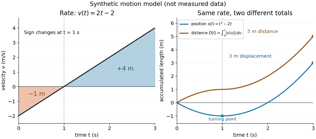
Synthetic variable velocity model with displacement 3 metres and distance traveled 5 metres over three seconds
. Details. 
Orientation matters independently of whether the integrand is positive or negative. For a function integrable on the interval containing the endpoints, use the conventionsFor the preceding velocity model, accumulation from seconds back to seconds gives m. Reversing the bounds of the speed integral gives m, which is an oriented integral, not a negative distance traveled from velocity; physical elapsed-time totals use the earlier endpoint first. The splitting rule holds even when is outside the interval between and , provided integrability holds on the interval containing all three endpoints.[ref]
Existence needs hypotheses. For a bounded function on with , a finite Riemann integral exists when every tagged Riemann sum approaches the same value as the largest cell width tends to zero:The limit must be independent of both the partition of an interval and the tags. Merely making the number of cells large can leave a wide cell unresolved. On a finite closed interval, every continuous function, and every bounded function that is continuous except at finitely many points, is Riemann integrable.[ref] Boundedness alone is insufficient: the Dirichlet function on is on the rational numbers and on the irrational numbers. Tags can all be chosen rational or all irrational, giving Riemann sums of or at arbitrarily small cell widths.[ref]
For a finite signed Lebesgue integral, the condition is instead that be a measurable function for Lebesgue measure and . A measurable function for Lebesgue measure that is also a bounded function on a finite interval satisfies this condition since gives . The Dirichlet function therefore has Lebesgue integral zero: the rational numbers form a null set, so it equals zero Lebesgue almost everywhere. The Riemann integral and Lebesgue integral agree for the continuous functions used in the diagrams.[ref]
Lecture 12: Lebesgue Integrable Functions, the Lebesgue Integral and the Dominated Convergence Theorem. Definition 120, Proposition 123(2), Remark 124 and Theorem 126
An unbounded integrand or infinite endpoint requires further analysis, for example the limits defining an improper integral; the notation alone does not establish convergence. Signed area under a graph 2026-10-14
For and a real-valued function with a finite Riemann integral or Lebesgue integral on , the signed area under a graph is its definite integral: geometric area above the horizontal axis contributes positively, and geometric area below it contributes negatively. If these two nonnegative areas are and , thenThe second expression is the total geometric area under a graph. Taking the absolute value of the first expression does not usually give the second: cancellation has already removed information about how much area lies on each side.[ref]
For an exact example, take the polynomial function on . Its polynomial roots are and : it is negative between them and positive on the two outer intervals. An antiderivative is , so the fundamental theorem of calculus givesThus and . The signed area under a graph is , whereas the total geometric area under a graph is . To compute the latter with antiderivatives, split at each sign-changing polynomial root and reverse the sign of the negative contribution.
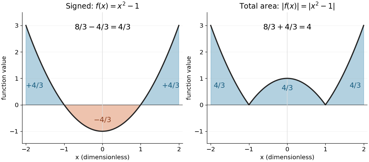
The polynomial x squared minus one has signed integral 4/3 and total geometric area 4 on the interval from minus two to two
. Details. 
Cancellation is useful information when the integrand represents a signed contribution. For the polynomial function on , the two triangular areas give , although . Zero net signed area therefore means balanced positive and negative contributions, rather than an empty region.
The short algebraic justification uses the positive part and negative part : and . Their integrals give and , and linearity of integration gives the difference and sum formulas. For Lebesgue integration, require both contributions to be finite to avoid the undefined subtraction .[ref]
Linearity of integration Created 2026-10-14 Updated 2026-10-20
For integrable real-valued functions on a measure space and fixed real numbers , their linear combination is integrable, and the Lebesgue integral satisfiesThe same rule applies to any finite summation: for integrable functions and fixed scalars . Finite signed values matter: integrability ensures all these integrals are finite, so no undefined occurs.
This is the distributive property of finite summation carried into integration: a fixed factor can be pulled out, and a finite sum can be integrated term by term. For simple functions, distribute the finite sums of value times measure; approximation extends additivity to nonnegative measurable functions, and splitting into a positive part and negative part gives the integrable signed case. See Lecture 12: Lebesgue Integrable Functions, the Lebesgue Integral and the Dominated Convergence Theorem (Proposition 122: linearity for integrable functions). For example, . With a probability measure, linearity of integration gives linearity of expectation.
Average value of a function Created 2026-10-14 Updated 2026-10-18
For an integrable function on an interval of positive finite length, its average value is the integral divided by that length:If is constant on equal-length subintervals, this is their values' arithmetic mean; unequal lengths require a weighted mean. For example, values and on two equal halves give average value , whereas value on the first quarter and on the remaining three quarters give . The integral measures total contribution; the average value of a function divides out the interval length.
For the function on , the average value of a function is . Replacing it by the constant preserves its integral on this interval. This is why the Haar projection uses cell averages to obtain a coarser description while retaining each cell's total contribution.
Bernoulli corrections for polynomial sums 2026-10-14
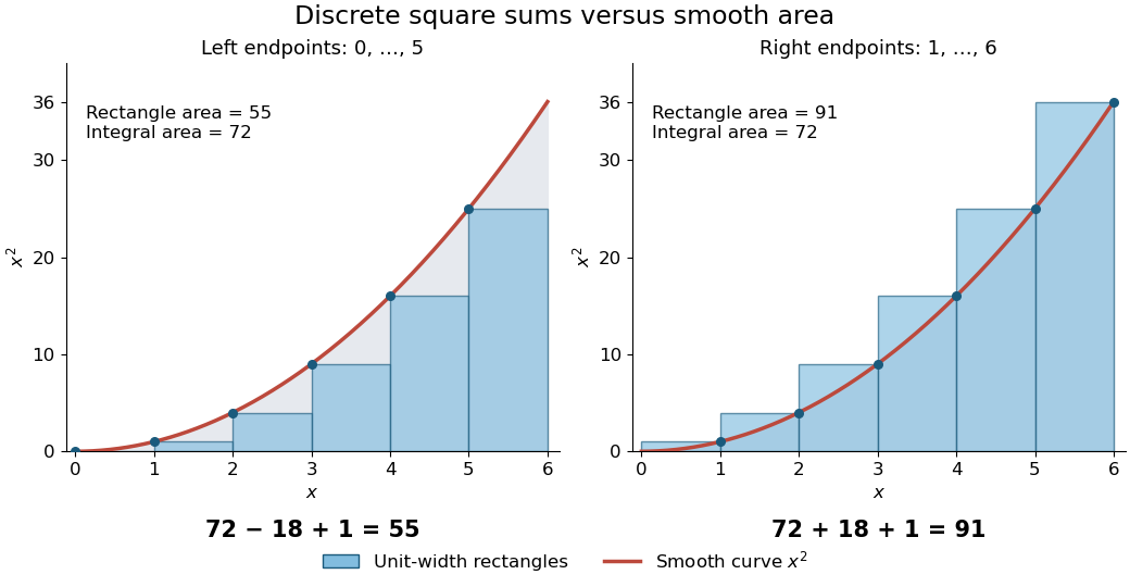
For a concrete comparison, take on . The integral is , whereas the unit-width left and right Riemann sums are and . The exact integer power sum formula givesThe endpoint choice explains the opposite signs of the correction. The remaining correction is one in both cases.

The same method is useful far beyond squares of numbers. Substituting , , and into the integer power sum formula gives the exact fourth-power resultAt , this isThus a finite polynomial calculation replaces ten additions, or a million additions if is a million. Although the individual corrections can be rational numbers, the result is the exact integer sum.
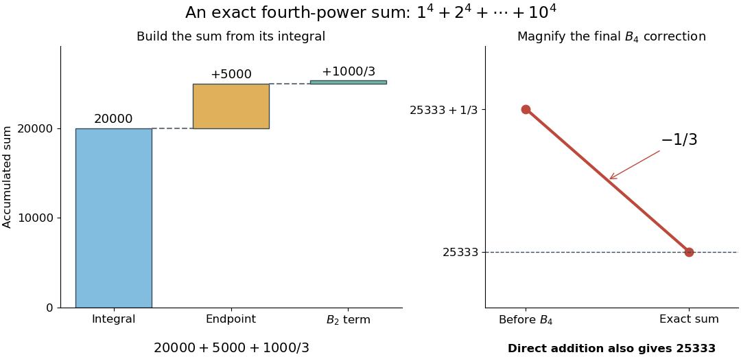

There is also a useful numerical integration interpretation. The average of the left and right Riemann sums is the composite trapezoidal rule. For , the endpoint corrections cancel but its value is , one above the true integral. Subtracting the correction makes this particular polynomial example exact. For , the two interior corrections above can be written and . These are exact identities for these polynomials; extending such corrections to general functions requires a separate error analysis.
Insulin receptor substrate 2026-10-14
An insulin receptor substrate is a docking protein phosphorylated by the activated insulin receptor. Its phosphotyrosine residues recruit downstream signaling proteins, including SH2 domain-containing components of phosphoinositide 3-kinase. This connects reception to the pathway described under insulin, rather than making the insulin receptor substrate another extracellular ligand.[ref]
Cell signaling by receptor-tyrosine kinases by Mark A Lemmon and Joseph Schlessinger. “Linking RTK activation to cell signaling”: IRS docking proteins and Figure 3A
Euclidean bounce 2026-10-14
A Euclidean bounce is a finite-action Euclidean saddle associated with decay of a false vacuum. It returns to the same metastable vacuum at the two ends of Euclidean time, instead of joining two degenerate stable vacua. Its characteristic negative fluctuation direction produces the imaginary part associated with a decay rate; the leading semiclassical suppression is . Translation zero modes are treated as collective coordinates. It should not be confused with the stable double-well tunnelling instanton whose repeated crossings give a real level splitting.
The injective hull of a uniform module is uniform. An injective endomorphism of a uniform injective module splits its image, so its complementary summand must vanish and it is an automorphism. Consequently all nonunits are precisely the noninjective endomorphisms. Their nonzero kernels are essential; intersection of two such kernels is nonzero, making their sum noninjective. Composition on either side preserves noninjectivity, unless the other map is a unit, which merely transports the kernel. Thus the nonunits form the unique maximal ideal, and the quotient is a division ring.
Injective hull of an Ore domain Created 2026-10-14 Updated 2026-11-05
For a domain satisfying the left Ore condition, its division ring of fractions is an injective essential extension of the left regular module. For a homomorphism on a nonzero left ideal, choose . A common left multiple gives , hence ; right multiplication by extends it. The Baer criterion proves injectivity. Clearing a left denominator proves essentiality. The same calculation gives , with the opposite ring required because right multiplications compose in reversed order.
L2 initial condition Created 2026-10-14 Updated 2026-10-18
An L2 initial condition specifies a square-integrable initial function up to equality almost everywhere. It need not have pointwise nodal values or classical derivatives. L2-compatible initialization of grid data uses bounded averaging or projection, and evolution estimates use the relevant L2 norm.
There are unlisted articles, also show them or only show them.