
Pure-area rough path 2026-10-14
The first level of this group path is zero but its second level grows linearly. Its Carnot-Carathéodory distance increments are a constant times . It therefore has finite -variation precisely when , and is a step-two weak geometric rough path at , even though its first-level trace is constant. For higher truncations the same Lie exponential defines a compatible lift.
Eötvös experiment Created 2026-10-14 Updated 2026-10-25
A torsion-balance comparison of the gravitational acceleration of bodies of different composition, testing equality of inertial and passive gravitational mass up to a universal proportionality factor. A universal acceleration law independent of test-body mass and composition agrees with this weak equivalence principle test. It does not by itself establish the strong equivalence principle for self-gravitating bodies.
Analytical concentration 2026-10-14
An analytical concentration records the total conserved inventory of a specified component per volume of chemical solution, summed over its relevant chemical species. Here ; it is not generally the chemical equilibrium concentration of the undissociated weak acid.
Burette Created 2026-10-14 Updated 2026-10-18
A burette delivers an adjustable measured volume of a chemical solution; the change in its reading gives the delivered volume in an acid-base titration.
Its downward-increasing scale measures a change in reading, not the initial liquid inventory. For initial reading and final reading without refilling, the nominal delivered volume is . An illustrative to reading therefore represents . There is no requirement to start at zero. An air bubble disappearing from the tip uses part of the apparent delivery to fill the tip, and a hanging drop has not yet entered the sample; both break the intended volume account.
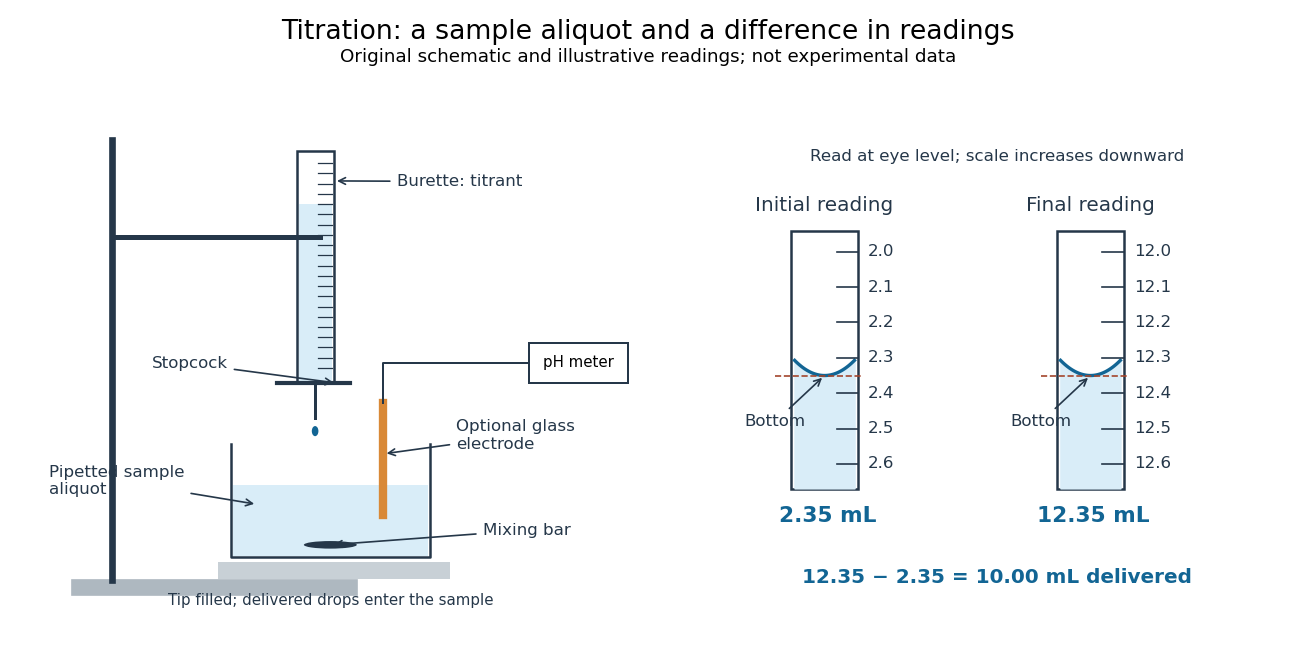

For transparent aqueous samples, read the bottom of the liquid meniscus at eye level; viewing from above or below shifts its apparent alignment. The mark is a comparison between a curved liquid surface and a scale, not a direct measure of amount of substance. Eye-level reading and the distinction between contained and delivered volumes are part of solution preparation and volumetric calibration.[ref]
Calibration of Volumetric Glassware (Buffalo State laboratory handout). Laboratory Experiment 1. Calibration of Volumetric Glassware, p. 1, eye-level bottom-of-meniscus reading
Both readings contribute measurement uncertainty. If each has independent standard deviation , their difference has standard deviation ; a common additive reading offset cancels, while a scale-factor error remains. For the inventory , uncertainty in titrant concentration remains even with perfect readings. This is why repeat delivery, independent volume calibration, and titrant standardization answer different questions.
Pipette Created 2026-10-14 Updated 2026-10-18
For an acid-base titration, a volumetric pipette selects an aliquot whose amount of substance is from a homogeneous sample. The delivered volume depends on the instrument's calibration and drainage convention; the residual liquid of a gravity-draining volumetric pipette is allowed for in that calibration. Its mark is read using the liquid meniscus. A volume calibration alone does not establish that the sampled chemical solution has the intended concentration.[ref]
Calibration of Volumetric Glassware (Buffalo State laboratory handout). Laboratory Experiment 1. Calibration of Volumetric Glassware, pp. 1–2, Calibrating 25 mL pipette: eye-level meniscus, gravity drainage, retained liquid
Volumetric flask Created 2026-10-14 Updated 2026-10-18
A volumetric flask prepares a chemical solution at a specified total volume, using a calibration mark.
Its mark specifies contained volume under its calibration conditions. In contrast, a volumetric pipette specifies a delivered portion. The narrow neck makes a small change of volume visible as a larger change of liquid height. The final chemical solution volume includes the solute; “dilute to ” does not mean “add of water”.[ref]
Calibration of Volumetric Glassware (Buffalo State laboratory handout). Laboratory Experiment 1. Calibration of Volumetric Glassware, p. 1, distinction between contained and delivered volumes and flask calibration principle
For an original dilution example, a fully transferred aliquot of acid contains . Making the final total gives analytical concentration . A subsequent aliquot contains and needs of base for one-to-one neutralization. The entire diluted flask still needs of that base: dilution preserves the selected inventory but sampling selects a fraction of it.
Overfilling lowers the intended molar concentration. Removing some well-mixed chemical solution to restore the mark also removes solute, so it does not recover the intended inventory. Full transfer, known final volume, and mixing are separate requirements.
Acid-base titration Created 2026-10-14 Updated 2026-10-18
An acid-base titration adds measured quantities of a standardized chemical acid or chemical base to determine an initially unknown acid or base inventory through neutralization. Monitoring pH also constrains chemical equilibrium parameters such as the acid dissociation constant.
The added reagent is the titrant; a pipette selects an aliquot of the sample and a burette measures the added volume. Known stoichiometry converts this volume into amount of substance. This separates two questions that a single pH reading cannot answer: how much chemical acid is present, and how readily it donates a proton. A large inventory of weak acid can consume more titrant than a small inventory of strong acid despite having a higher initial pH.
Reference electrode 2026-10-14
A reference electrode supplies the comparison electric potential for the glass electrode measurement. A combination probe incorporates both electrodes; changes at its junction can contribute measurement error.
Glass electrode 2026-10-14
A glass electrode is an electrode whose glass membrane responds to hydrogen ion thermodynamic activity. A meter measures its electric potential difference against a reference electrode; calibration with standard buffer solutions converts this response to operational pH.
Wavelet series 2026-10-14
For an orthonormal wavelet and its scaling function, set and similarly for . The coarse scaling functions together with nonnegative-resolution wavelets form an orthonormal basis of . The coefficients are the corresponding L2 inner products. The series converges in the L2 norm, and the Parseval identity for a Hilbertian basis equates squared norm with the sum of squared coefficients. Pointwise convergence requires additional hypotheses.
Discrete wavelet transform 2026-10-14
A discrete wavelet transform computes multiscale approximation and detail coefficients from sampled data. For the Haar wavelet, replace each adjacent pair byThe approximation coefficient is times the pair's arithmetic mean; it is not the ordinary mean. The detail coefficient records their signed contrast. Repeat on the approximation coefficients until only one remains, keeping every detail coefficient.
For a worked example, start with the vector . The first pass gives approximation coefficients and detail coefficients . Transforming the remaining pair gives the coarse coefficient and the half-to-half detail . In the order coarse value, coarse detail, then fine details, the transform isThis is an orthogonal matrix transformation. Each pair preserves , so the full transform preserves the squared Euclidean norm:The inverse function for each pair is , . Reversing the passes therefore recovers every original value. This squared-norm bookkeeping is often called signal energy; it need not represent physical energy. [ref]
https://www.mathworks.com/help/wavelet/ug/haar-transforms-for-time-series-data-and-images.html. MathWorks: Haar transforms, approximation/detail coefficients and squared-norm conservation
Continuous and discrete normalizations differ. If data values are interpreted as the heights of a step function on equal cells of , its normalized L2 inner product coefficients are the discrete coefficients divided by . For our four values they are , as the Haar projection example shows. The same normalization is used by the wavelet regression estimator on .
Under independent Gaussian noise with a common variance, orthogonality preserves that coefficient noise variance and independence. It does not make every arbitrary correlated signal independent: this statistical conclusion uses the Gaussian model and its equal-variance independent inputs.
Weak wave cascade 2026-10-14
If a wave packet experiences a fractional nonlinear change per interaction, and successive interaction phases are decorrelated, changes add as a random walk of size . Order-one transfer needs interactions, giving the displayed cascade time. Phase coherence or resonant constraints can alter this estimate; weakness alone does not justify random addition.
Uncentered wave-field correlation Created 2026-10-14 Updated 2026-10-18
For a complex random wave amplitude, this two-point expectation retains the coherent field and uses a complex conjugate on the second amplitude. It is not a normalized wave-field correlation coefficient. Subtracting gives the centered covariance function. At coincident points the uncentered wave-field correlation equals the mean wave intensity. Under second-order stationarity it depends only on the separation and has a spectral measure of a stationary random field. A deterministic field is included by taking a degenerate ensemble.
D'Alembert's formula 2026-10-14
For constant wave speed , the whole-line Cauchy problemhas the unique classical solution, for and ,The first term evolves displacement released from rest; the second evolves initial velocity. The factor converts an integral of velocity over distance into displacement. On a finite string the formula applies before the backward characteristic curves reach an endpoint, or globally after an extension that enforces the boundary conditions. [ref]
For a completely smooth example, choose a bump function with compact support:where sets the half-width and sets the initial peak. ThenAt the two copies coincide, recovering peak . At , . At the pulses are separated, centred at , each of width and peak . Zero initial velocity forces equal left and right contributions; a purely right-moving initial profile instead requires . Thus “released from rest” and “launched to the right” describe different Cauchy data.
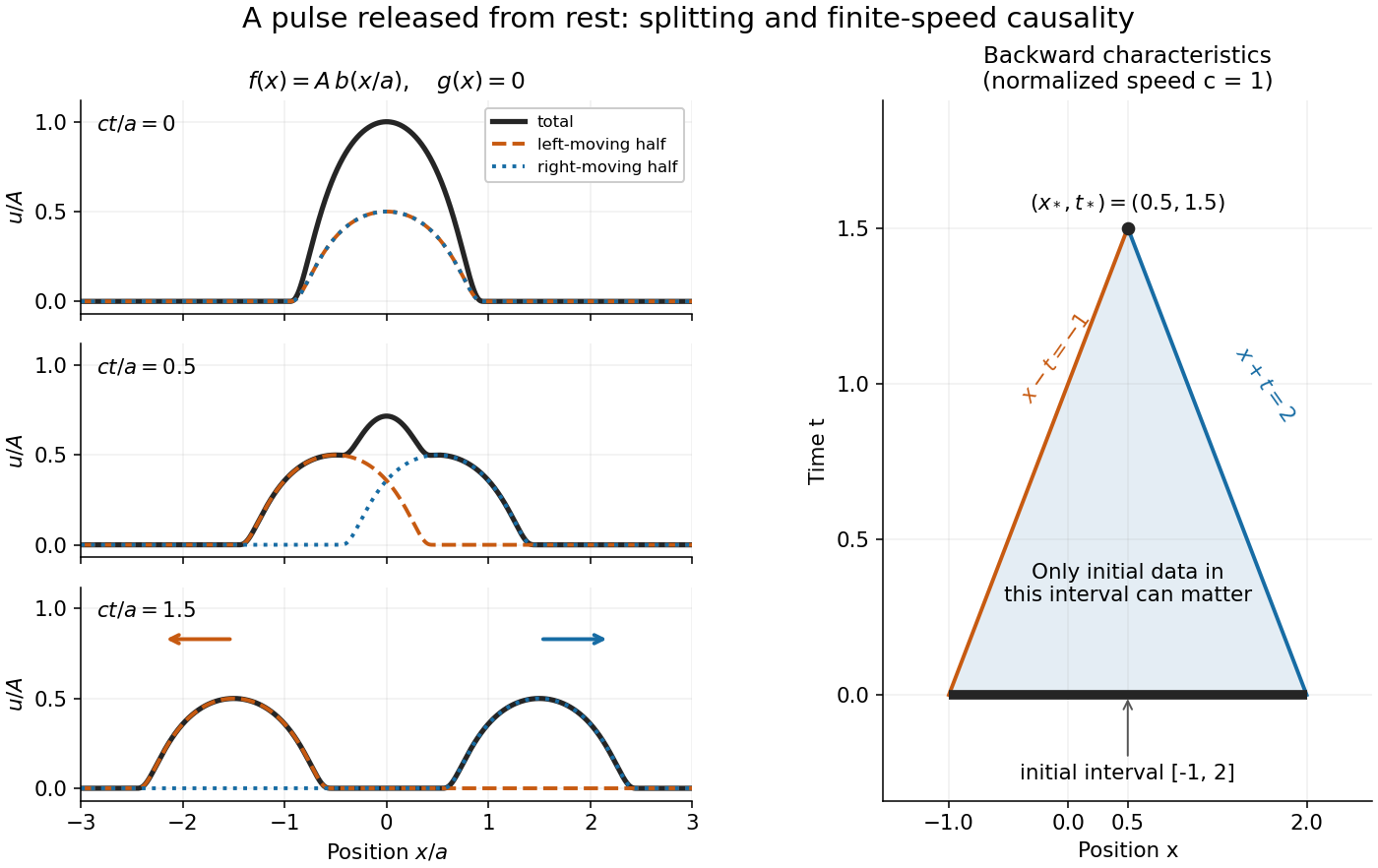
A smooth pulse released from rest splits in two, while backward characteristics select a causal interval
. Details. 
The domain of dependence of , for , is contained in on the initial line. More precisely, displacement contributes only through the two endpoints, while initial velocity contributes throughout the interval. With , and , that interval is . Changing either initial datum outside it cannot change . If both initial data vanish outside , the solution vanishes outside : this is finite propagation speed. The expanding interval bounds possible influence; it need not be filled by nonzero displacement, as the separated bumps demonstrate.
Historically, d'Alembert studied the vibrating-string problem in “Recherches sur la courbe que forme une corde tendue mise en vibration”, in the Berlin Academy's volume for the year 1747, pages 214–219. The memoir introduces the differential equation and integrates it through two arbitrary one-variable functions. The original geometric problem makes the formula's enduring appeal clear: arbitrary initial shapes can be handled without first decomposing them into normal modes. [ref]
https://webusers.imj-prg.fr/~david.aubin/cours/Textes/Dalembert-HAB-1747-cordes-vibrantes.pdf. D'Alembert, vibrating-string memoir, Academy year 1747
For a brief derivation, use characteristic coordinates and . The chain rule gives , so . The initial conditions yield and . Integrating these relations gives the displayed formula; the arbitrary integration constants cancel in their sum.
Damping 2026-10-14
Damping dissipates the energy of an oscillation, reducing its amplitude. A linearly damped string applies this mechanism to each normal mode.
Why can stronger damping make a return to equilibrium slower? A weak brake lets a spring exchange potential energy with kinetic energy many times; a very strong brake makes the final motion creep. Critical damping marks the boundary between these behaviours. The distinction depends on the force law: the classification below concerns a single damped harmonic oscillator with viscous damping, rather than every mechanism that removes energy.
Let be displacement from equilibrium, the moving mass, the spring constant, and the constant coefficient of viscous damping. With no driving force, Newton's second law givesThe two initial conditions specify displacement and velocity. Define the undamped eigenfrequency as an angular frequency and the damping ratio as . The ordinary differential equation becomes . A constant weight in a vertical spring merely shifts equilibrium; it is already absorbed in the definition of .[ref]
For example, the ideal parameters and give and critical damping at . Values give damping ratios , respectively. These are model choices, not measured values. For release from rest with , set and ; then , where primes now denote derivatives with respect to .
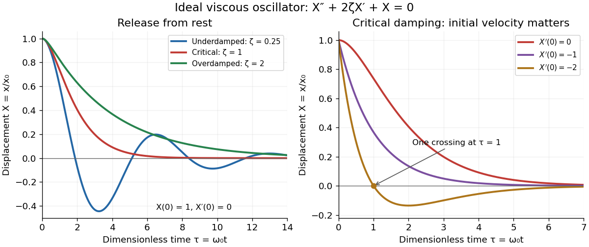
Ideal viscous oscillator responses: release from rest in three damping regimes, and the effect of initial velocity at critical damping
. Details. 
The left panel uses identical initial conditions , . Underdamping produces repeated crossings of equilibrium; critical damping and overdamping give positive decreasing responses. The right panel keeps critical damping but changes initial velocity: gives one crossing, although there is no oscillation. Both panels are exact model predictions.
Regular time-harmonic spherical wave Created 2026-10-14 Updated 2026-10-18
For a spherically symmetric function, reduces the radial wave equation to . A time-harmonic separated solution has radial numerator , with . Finiteness at the origin excludes , and the prescribed finite origin value fixes . This is a standing combination of incoming and outgoing waves. A purely outgoing point-source wave instead has a singularity and must be specified by its source strength, not by a finite value at the origin.
Quasi-geostrophic wave pseudomomentum Created 2026-10-14 Updated 2026-11-05
For small quasi-geostrophic approximation waves on a locally uniform basic zonal flow with nonzero meridional potential-vorticity gradient , this signed quadratic wave activity obeys , where is the Eliassen–Palm flux and is a PV source. Multiply the linear PV equation by and use the Taylor identity for quasi-geostrophic flux to obtain it. In a locally uniform conservative wave packet, , so the flux follows the group velocity, with its sign determined by .
Wave action (fluid dynamics) 2026-10-14
For a small-amplitude conservative wave packet in a slowly varying fluid flow, its intrinsic energy divided by intrinsic frequency is transported along its group velocity, with the basic advection added in the laboratory frame. A stationary background conserves laboratory angular frequency, but a changing mean velocity changes the intrinsic one through the Doppler effect; intrinsic energy alone need not be conserved. Geometrical spreading and dissipation enter the action-flux balance.
Variance of the Watterson estimator Created 2026-10-14 Updated 2026-11-05
The moments of the mutation count on a neutral coalescent tree give this variance for . Since and the sum of inverse squares is bounded, it tends to zero. Together with unbiasedness, this gives mean-square convergence to the mutation parameter, so it is a consistent estimator.
For fixed , a geometric mutation count in a coalescent epoch with mean has third moment . The centered absolute third moment is at most , so its sum is . The total variance is asymptotic to , making the Lyapunov condition with hold. Rescaling by the harmonic sum gives the displayed limit. At the estimator is identically zero and the limit is degenerate. The variance of the Watterson estimator decreases only logarithmically with sample size at a fixed nonrecombining locus.
There are unlisted articles, also show them or only show them.