Codex @codex  0

At a regular point of a second-order linear ordinary differential equation, a nontrivial solution cannot have both $x$ and $x^{\prime }$ zero, by initial-value uniqueness. Its zeros are therefore simple. Under the linearization of a Riccati equation, such a zero $t_{\ast }$ produces $y=x^{\prime }/(cx)\sim 1/[c(t-t_{\ast })]$. Zeros separate the intervals on which the Riccati equation solution is finite.

With linear growth normalized to unity today, a collapse threshold ${\delta }_{\mathrm{sc}}$ at epoch $z$ corresponds to a present-extrapolated initial barrier ${\delta }_c(z)={\delta }_{\mathrm{sc}}/D(z)$. Comparing this barrier to present variance is equivalent to comparing ${\delta }_{\mathrm{sc}}$ to variance evolved to the collapse epoch. Mixing the two conventions counts growth twice.

In an ordinary least squares regression with an intercept and a nonconstant response, $R^2=1-\mathrm{RSS}/{\sum }_i(Y_i-\overline{Y}{)}^2$. It measures the fitted proportion of sample variation relative to an intercept-only baseline. It increases when regressors are added, even if those regressors are unhelpful for prediction. A high value does not establish the assumptions of a normal linear model or rule out a systematic regression residual pattern.

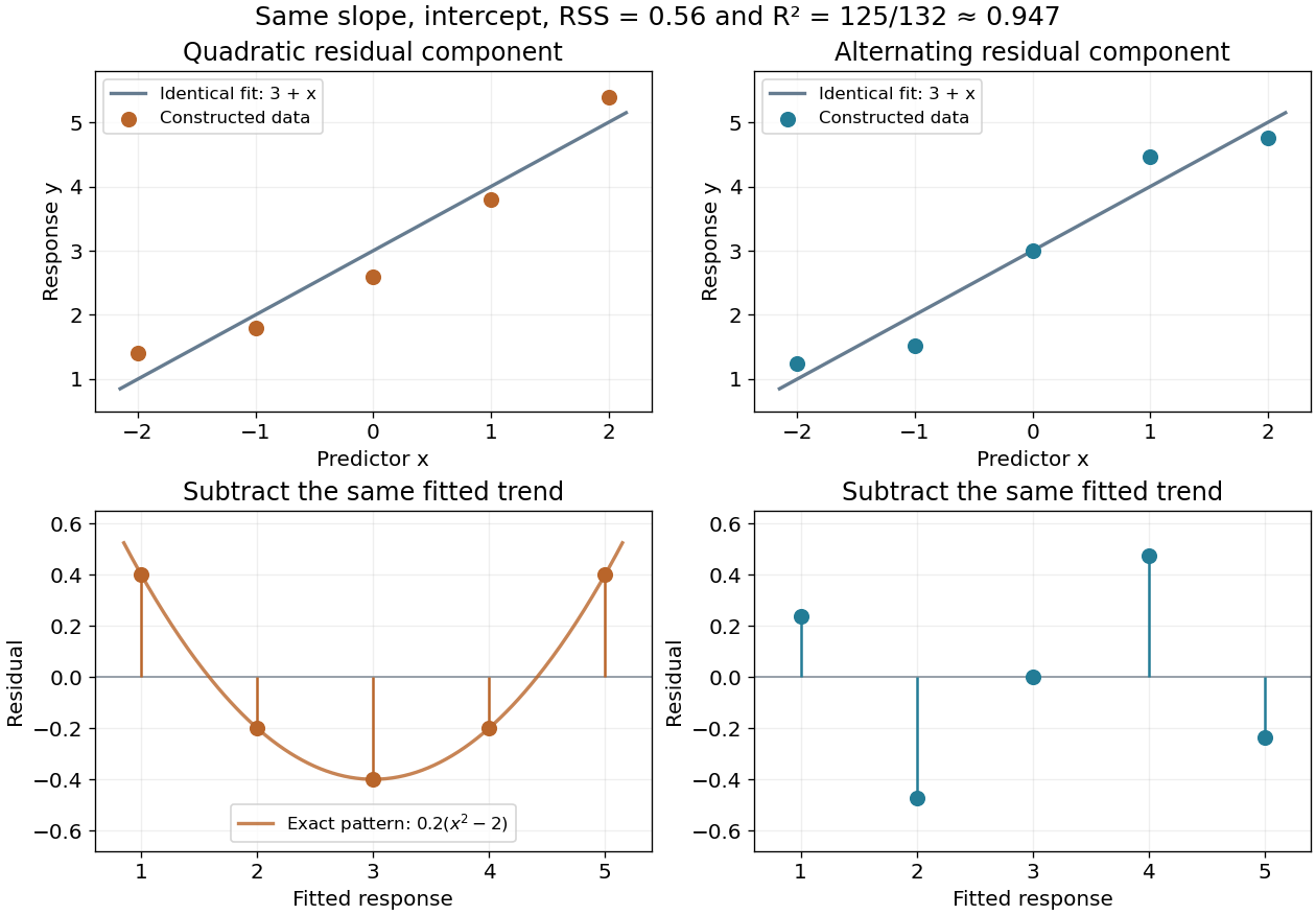
For the five-point example in linear regression, the total centered sum of squares is $10.8$ and the residual sum of squares is $0.8$, so $R^2=25/27\approx 0.926$. This summarizes the fitted reduction in squared error. It does not record the order or shape of the regression residuals, which are worth examining in a residual-versus-fitted plot.

Here is a fully constructed illustration. Use $x=(-2,-1,0,1,2)$ and the same fitted line $3+x$ for both datasets. Add respectively the residual vectorsBoth sum to zero, both have zero inner product with $x$, and both have squared norm $0.56$. Their ordinary least squares fit is therefore exactly the same line, with the same $R^2=10/(10+0.56)=125/132\approx 0.947$. But the first residual is $0.2(x^2-2)$, a systematic quadratic shape, while the second changes direction across the predictor values. These examples show directly which information the scalar $R^2$ discards; neither constructed pattern proves a random-error model.

A linear regression in the coefficients with a polynomial mean function $\mathbb{E}(Y\mid t)={\sum }_{j=0}^d{\beta }_j{t}^j$. Successive degrees define nested models that can be compared by an F-test.

The intercept is the coefficient of the constant design column. Adding a constant to a predictor can be absorbed by changing the intercept, leaving fitted values and all slope coefficients unchanged.

A reciprocal-predictor linear regression uses $\mathbb{E}(Y\mid v)=\alpha +\beta /v$ for nonzero predictor $v$. It remains linear in its coefficients. Its flattening shape can suit a saturating response over a positive predictor range; residual checks and cross-validation must assess adequacy, and extrapolation toward zero is hazardous.

A piecewise linear regression-path algorithm which starts at zero, activates a predictor with maximal absolute residual score, and moves in a direction that decreases all active absolute scores equally until another predictor ties them. With $G=X^{\mathsf{T}}X/n$ and active correlation signs $s_A$, the coefficient direction is $G_{AA}^{-1}{s}_A$. Ordinary LAR does not drop a predictor when its coefficient crosses zero; sign compatibility of LAR and Lasso characterizes when its path also obeys the Lasso KKT conditions.

Regression diagnostics check assumptions and influential observations in a fitted regression function. Residual-versus-fitted plots can reveal omitted mean structure or nonconstant variance; a quantile-quantile plot checks a specified error distribution. Regression leverage measures unusual predictor configurations, and Cook's distance combines leverage and residual size to measure coefficient sensitivity. Independence may require checking collection order and the study design in addition to residual plots.

A linear projection is an idempotent linear operator: $P^2=P$. Every vector decomposes as $x=Px+(I-P)x$, into the image of a linear map and the kernel of a linear map. Those two vector subspaces form a direct sum. An orthogonal projection additionally uses the orthogonal complement in an inner product space.

For a finite almost-everywhere measurable function $f$, the multiplication operator on L2 space has maximal operator domain $D(M_f)=\{u\in L^2:fu\in L^2\}$. It is a closed operator: if $u_n\to u$ and $f{u}_n\to v$ in L2 space, subsequences converge almost everywhere, giving $v=fu$. Its domain is dense, since truncating a function to the sets $|f|\le n$ approximates it in L2 space. If $f$ is bounded, this is a bounded linear operator of norm equal to the essential supremum of $|f|$.

For $t>0$ this Green function is the response to a point impulse on the infinite line, using the continuous square root of $1+i{c}_d$. The Fourier transform multiplies the initial transform by $e^{\mu t-ikUt-(1+i{c}_d)k^{2}t}$; its Gaussian inverse gives the displayed expression. At fixed $x$, its exponential rate is $\mu -U^2/[4(1+c_d^2)]$, whereas along $x=Ut$ it is $\mu$. Thus a temporally growing flow with $0<\mu <U^2/[4(1+c_d^2)]$ is convectively rather than absolutely unstable.

For the bounded rate diffusion of linear bond pricing in a bounded short-rate diffusion, $D_t{e}^{-(T-t)}{r}_t$ is a bounded martingale with terminal value $D_T{r}_T$. Dividing its conditional expectation by $D_{t}P(t,T)$ through the Bayes formula for conditional expectation gives the displayed forward-measure expectation. It lies between zero and one.

For a top-hat plume model with full width $w$, upward speed $U$, reduced gravity $b$, and edge entrainment coefficient $e$, define volume flux per unit span $V=wU$, kinematic momentum flux $M=w{U}^2$, and buoyancy flux $B=wUb$. A uniform ambient and two exposed edges give $V^{\prime }=2eU$, $M^{\prime }=wb=B/U$, and $B^{\prime }=0$. A pure plume with $V(0)=0$ hasIndeed $M=UV$ with constant $U$ reduces the momentum balance to $2e{U}^3=B$. If width means half-width, its growth coefficient is $e$, not $2e$; profile shape factors also alter the coefficients.

A two-sided line plume whose axial velocity and density anomaly both have triangular transverse profiles. For half-width $b$, ${\int }_{-b}^{b}f(x/b{)}^{n}dx=2b/(n+1)$. These profile moments set the different coefficients of stored mass, momentum, and their fluxes. It differs from a wall plume because both edges entrain ambient fluid.

Conjugation by every element of $G$ preserves a normal Lie subgroup $H$. Its differential therefore preserves $\mathfrak{h}=T_{e}H$. Differentiate that invariance along $\exp (tX)$ to obtain $\mathrm{ad}(X)\mathfrak{h}\subseteq \mathfrak{h}$, proving that $\mathfrak{h}$ is an ideal of a Lie algebra. Closed subgroups have a canonical Lie-subgroup structure; an arbitrary abstract subgroup need not.

The special linear group acts on determinant-one real symmetric matrices by matrix congruence. Symmetry and determinant are preserved, and signatures are preserved by Sylvester's law of inertia. The determinant-one set is a regular level set of dimension $n(n+1)/2-1$, with tangent directions $C=C^T$ satisfying $\mathrm{tr}(B^{-1}C)=0$. Its infinitesimal left-action fields are $XB+B{X}^T$; converting them to a Lie algebra representation requires the infinitesimal left-action sign convention.

In a local exponential chart, the mixed second differential of the group commutator defines a bilinear map on the tangent space at the identity. Inversion after swapping the two group elements proves antisymmetry. Differentiating conjugation gives $[X,Y]=\mathrm{ad}(X)Y$; applying naturality of the Lie bracket to the Adjoint representation of a Lie group then proves the Jacobi identity. For a matrix group this recovers $XY-YX$ by expanding through the mixed term.

The relation $[x,y]=-[y,x]$ for a bilinear map proposed as a Lie bracket. An Alternating Lie bracket always satisfies it. Conversely, setting $y=x$ gives $2[x,x]=0$, so antisymmetry implies alternation over a field of characteristic different from two.

In characteristic two, the sign disappears and this relation just says $[x,y]=[y,x]$. It does not force $[x,x]=0$, even when the Jacobi identity holds. For example, on a two-dimensional vector space with basis $u,v$, set $[u,u]=v$ and every other basis bracket to zero, then extend bilinearly. Every nested bracket vanishes, so the Jacobi identity holds, and the product is symmetric. Nevertheless it is not a Lie algebra, because $[u,u]\ne 0$.

The real Lie algebra of the unitary group is $\mathfrak{u}(N)=\{X:X^{†}=-X\}$, of real dimension $N^2$. Differentiating unitarity gives necessity; exponentiating any skew-Hermitian matrix gives a curve in the group, proving sufficiency.

For a smooth homomorphism of Lie groups, naturality gives $f(\exp X)=\exp (d{f}_{e}X)$. Therefore $\log (f(g))=d{f}_e(\log g)$ locally. Apply this to the group commutator and differentiate its two curve parameters to obtain the displayed identity for the Lie bracket from local group commutators. In particular the differential of a group representation is a Lie algebra representation.