
Past exam of the mathematics course of the University of Cambridge 2004 iii Paper 53 1 Solution Created 2026-10-03 Updated 2026-10-14
Write for the controlled unitary gate. For a normalized eigenvector , the first Hadamard gate and quantum phase kickback giveThe final Hadamard gate therefore produces the unentangled outputThe auxiliary system is unchanged, while its eigenphase becomes accessible through interference of the control qubit. The special unitary group assumption is not needed for this calculation; unitarity and the normalized eigenvector suffice.
Past exam of the mathematics course of the University of Cambridge 2004 iii Paper 51 4 Solution Created 2026-10-03 Updated 2026-10-14
Interpret triviality as holomorphic triviality. Choose a global holomorphic bundle frame for . Let have as its columns the coordinates of these sections in the prescribed local frame over , with the convention that a fiber coordinate vector transforms as . ThenEach is holomorphic and invertible because its columns form a basis in every fiber. This proves the requested holomorphic splitting of transition functions on a trivial bundle. Smooth or topological triviality alone would not justify holomorphic splitting.
For the line bundle on projective twistor space, pull its patching function back to the twistor line using the incidence convention of this problem, , without an extra factor of . Triviality on each line gives nonvanishing linewise holomorphic functions with . The factors can be chosen as holomorphic functions of locally: a degree-zero scalar transition function has zero winding on the overlap annulus, hence admits a logarithm there; splitting its positive and negative Laurent series parts gives factors whose coefficients are Cauchy integrals that are holomorphic functions of . The explicit splitting is worked out below. Their only common linewise ambiguity is multiplication by a nonzero function : the ratio is a global holomorphic function on the compact complex projective line, hence constant on that line.
Take , and raise a two-component spinor by left multiplication with . The derivative along an alpha-plane is . It annihilates the unsplit twistor function, becauseThusis holomorphic on the whole line and has projective weight one. A section of is linear in the homogeneous coordinates: in an affine coordinate, holomorphic regularity at infinity bounds its growth to at most first order, so the Cauchy integral formula excludes all higher powers. ThereforeThe inverse splitting functions obey . Commuting these two equations provesThe spinor decomposition of gauge curvature iswhere both two-component spinors are symmetric. Vanishing of the contraction for every forces . This is exactly the anti-self-dual Maxwell equations. Since the Abelian gauge curvature is , it is closed; its duality condition also makes it co-closed, giving the source-free Maxwell equations. Changing both splitting factors by changes by , the expected Abelian gauge transformation. This derives the rank-one Penrose-Ward correspondence in the needed local form.
For the exponential patching function, choose a representative of the Čech cohomology class, of homogeneous degree zero. On the overlap of the two line patches write . To compute the gauge potential explicitly, use a constant two-component spinor basis in which and the finite patch . Then , andFor a positively oriented contour in the overlap annulus, split its Laurent series asThe first is holomorphic inside the contour, the second outside including infinity; split . Since , coefficient comparison gives . Applying that operator separately to cancels all nonconstant terms and leavesThus yields and . MoreoverSubstitution gives , which in homogeneous form is preciselyThis is the Abelian Ward splitting by Laurent series. The factors have weights , respectively, so the integrand is invariant under a change of homogeneous representative. The contour avoids ; the basis chosen above places that point at infinity. One can keep the contour fixed for in a sufficiently small domain, allowing differentiation under the integral.
Finally differentiate the contour potential for an anti-self-dual Maxwell field. By the twistor incidence relation, . ConsequentlyThe second equality uses the elementary two-spinor identity in the declared convention. The remaining two-component spinor is symmetric in , and no primed symmetric gauge curvature part survives. This directly verifies is anti-self-dual. In complexified Lorentzian signature duality has Hodge star eigenvalues ; here the vanishing primed two-component spinor fixes the stated ASD convention rather than incorrectly imposing the Euclidean equation on that signature.
Past exam of the mathematics course of the University of Cambridge 2004 iii Paper 51 3 Solution Created 2026-10-03 Updated 2026-10-14
Let and , using the oriented Euclidean metric. For a self-dual two-form ,Apply this componentwise in the Lie algebra. Since the three span the self-dual subspace, their vanishing wedges force . Thus . The gauge-theory Bianchi identity is , so , the Euclidean Yang-Mills equations. This proves the implication locally; finite action would additionally be needed to call the solution an instanton.
Use the complex orientation for and . The real and imaginary parts of , and , span the self-dual two-forms. Accordingly the three gauge curvature equations areFor a spectral parameter , consider the Lax pairTheir commutator isIt vanishes for every exactly when all three coefficients vanish. The derivative directions and are mutually orthogonal null vectors for the complexified metric. Flatness on the corresponding two-planes makes the linear parallel-transport equations locally compatible. Conversely compatibility for an invertible fundamental matrix forces the commutator to vanish; a single zero solution would not establish it. This is the Euclidean complex-coordinate anti-self-dual Lax pair.
For an Abelian U(1) connection, all commutators of the connection components vanish, and the gauge curvature equations therefore readLocally the first two equations say that is -closed and is -closed. The Dolbeault-Poincaré lemma, and its complex conjugate, give scalar functions withSubstituting in the third equation givesIn a complex gauge transformation, use and the derivative-plus-connection convention . ThenThis is the scalar Laplace equation, since for the stated metric . The complex gauge transformation need not remain in .
A reduction using only a unitary gauge transformation is also available. Since is anti-Hermitian, and , so the potential for the barred components can be chosen as . Write with real . Then , and removes the last term. With this givesIts gauge curvature is . Thus the Abelian anti-self-dual connections from harmonic scalar potentials reduction is local and does not require silently enlarging the real gauge group.
Past exam of the mathematics course of the University of Cambridge 2004 iii Paper 51 2 Solution Created 2026-10-03 Updated 2026-10-14
Use the Minkowski metric convention . On the Adjoint representation, the adjoint covariant derivative is . Set and . ThenThe trace obeys , and covariant integration by parts has the ordinary boundary term because the trace of a commutator is zero. Thus compactly supported variations giveThe trace pairing on is nondegenerate, so the Euler-Lagrange field equations areIn particular the sign of the scalar mass term follows from the plus sign in the supplied trace Lagrangian density; it should not be guessed from a different metric convention. This is the adjoint Yang-Mills-Higgs trace variation.
For the static Bogomolny-Prasad-Sommerfield monopole, take the usual purely magnetic extension and temporal gauge . At , the equations reduce towith the equation identically zero. We now verify both spatial equations from without assuming them. The gauge-theory Bianchi identity gives , hence immediately . Also , soHere . This proves that the Bogomolny equations imply all static zero-mass Yang-Mills equations and the scalar equation. The specification of matters: the spatial Bogomolny equations by themselves do not constrain an arbitrary extra electric potential, so the implication is for their standard purely magnetic static extension.
Past exam of the mathematics course of the University of Cambridge 2004 iii Paper 51 1 Solution Created 2026-10-03 Updated 2026-10-14
The canonical momentum is , so the Hamiltonian density and total energy areThe Euler-Lagrange field equation is . Multiplication by gives the local conservation of energy identityThus is conserved when the energy flux vanishes at spatial infinity. For finite energy with asymptotically constant fields, the endpoints must be scalar-field vacua, where .
Choose an antiderivative . For either sign , completing the square givesChoosing to make the boundary term nonnegative proves the Bogomolny boundThese Bogomolny equations obtained by square completion for a one-dimensional kink describe minima within a fixed endpoint sector when a saturating configuration exists. Differentiating the spatial equation gives wherever , with smooth extension to its limiting scalar-field vacua. The absolute minimum across all sectors is a constant zero-potential scalar-field vacuum when one exists; the nontrivial minima are sector-specific kinks.
For , write . The scalar-field vacua are . A static finite-energy solution has the first integralbecause differentiating its left side gives , and its value is zero at infinity. In either adjacent interval, . Set . The first-order equation becomes , with , and separation gives . HenceFor the endpoints are ; for they are . Thus there are four oriented static kink families, up to translation, namely two increasing kinks and two decreasing antikinks. Each has rest energyA static field joining directly to would have to pass through at finite . The first integral then gives , and the Picard-Lindelöf theorem applied to the smooth second-order equation with those initial conditions forces . Therefore there is no such additional kink; this is the intermediate-vacuum obstruction to a kink. The Bogomolny classification of a rescaled phi-six kink also shows that if , only the scalar-field vacuum remains and there is no nontrivial finite-energy static kink. Indeed the first integral gives a monotone field wherever it is nonzero, precluding a return to the same scalar-field vacuum.
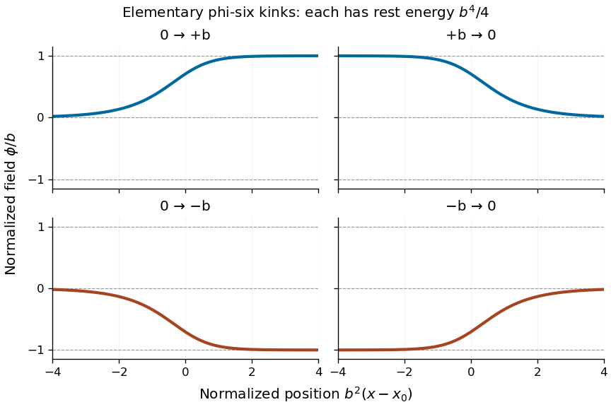
Four oriented elementary phi-six kink profiles connecting adjacent vacua, with equal rest energy
. Details. 
A Lorentz boost of the profile gives a moving solution with arbitrary :If denotes the static profile and , then , proving the Euler-Lagrange field equation directly. Its energy is : since , changing variable to in the energy integral gives the factor . Reversing or yields the other moving elementary profiles.
Past exam of the mathematics course of the University of Cambridge 2004 iii Paper 50 6 Solution Created 2026-10-03 Updated 2026-10-14
Work on the physical domainand abbreviate , , and . There are no vector multiplets specified, hence no additional gauge D-term. In Planck units the supergravity F-term potential and upper-index supergravity auxiliary fields areThe overall auxiliary-field sign is a convention; its vanishing and norm are invariant statements.
The Kähler covariant derivatives of a superpotential here areThe Kähler metric, with rows and columns their barred partners, isIts block is positive definite because its leading diagonal and determinant are positive. In the inverse-tensor convention , the nonzero upper components areIn particular the conjugations in the off-diagonal components matter.
To verify the no-scale supergravity cancellation explicitly, temporarily write and . Their part of the metric contraction isThe terms involving and its conjugate cancel between the mixed and diagonal contributions. The remaining cancels the universal negative term. Since , the exact matter-logarithm no-scale potential is thereforeIt differs from a model where appears outside the logarithm in the Kähler potential.
Substitution into the auxiliary-field formula givesFor example , which reduces to the displayed expression for the cubic superpotential. To test unbroken supersymmetry at any finite point, first forces . Then forces , whereas forces . Subtracting gives . Because , and at a finite point, all auxiliaries can vanish only if . Thus every nontrivial choice of breaks supersymmetry at finite field values.
A finite zero-energy minimum requires both nonnegative terms of to vanish:There cannot be a finite positive-energy stationary point: keeping fixed and varying the real part of , equivalently , giveswhich is strictly negative unless . Hence these zero-energy solutions are all the possible finite minima.
Because were allowed to be arbitrary, existence must be checked. If both are nonzero, put and . The magnitude equation isThe function on the right starts at one at the excluded boundary , tends to zero as , and has derivative . Its maximum is at . Therefore a finite cubic-matter no-scale vacuum with an exponential dilaton exists exactly whenThere is one finite positive root for , two for , and one merged root at the maximum. The complex phase equation fixes modulo . If exactly one of vanishes, or the ratio exceeds the bound, no finite minimum exists; the potential instead has infimum zero along the runaway . A zero infimum at an infinite-field boundary is not an attained finite vacuum.
On a nontrivial finite branch, , soThis proves supersymmetry breaking at the intended no-scale vacuum. Its zero energy is consistent with the negative gravitational term: , which cancels in . It is not a counterexample to the global-supersymmetry positivity argument in question 3.
Both real components of are exactly flat on the vacuum family: never enters the potential, and at every allowed positive gives the same zero energy. Generically both components of are fixed. Although the matter field has no quadratic mass there, it is not an exact flat direction: for fixed at its root, and the leading positive potential is . At the special merged root , the real- quadratic curvature also vanishes, but higher orders lift it; this does not add a continuous flat vacuum direction. If , by contrast, is a supersymmetric zero-energy family with both complex and flat and all auxiliaries zero. This exception prevents an unconditional breaking assertion for arbitrary constants.
Finally the gravitino mass from a superpotential isAt a nontrivial finite minimum it becomesIts value varies along the flat volume modulus; the classical potential does not select a unique supersymmetry-breaking or gravitino-mass scale. On the trivial supersymmetric branch , it is zero.
Past exam of the mathematics course of the University of Cambridge 2004 iii Paper 50 5 Solution Created 2026-10-03 Updated 2026-10-14
Start with the Clifford algebra . For the dimension count, complexify and rescale the timelike matrix so that the generators obey the Euclidean complex relation . This changes neither the complex representation dimension nor its decomposition under the complexified even algebra. In , pair the generators intoDirect substitution gives and . The commuting operators satisfy , so their occupation eigenvalues are zero or one. An irreducible module contains an all-zero occupation state , obtained by lowering the occupied entries of a simultaneous eigenvector. The statesare nonzero and independent by their distinct joint occupation eigenvalues. They span an invariant module; irreducibility makes this the full module. Conversely this Fock construction supplies a representation on exactly these states. Products of occupation projectors and raising/lowering operators give its matrix units, so the generated algebra is the full matrix algebra. Therefore the minimal complex Dirac spinor has
This module is irreducible under the full Clifford algebra, but the Spinor representation of the Lorentz group is generated by the even bilinears . The chirality matrix in the Euclideanized basis isIts two eigenspaces therefore remain invariant under Lorentz transformations. Each has half the Fock states, since any gamma matrix bijects them. The even algebra connects every pair of occupation states of the same parity and has no further invariant subspaces within either one. HenceThese are the irreducible Weyl spinors. Globally they are ordinary representations of , the double cover; calling them representations of uses the conventional projective spinor terminology.
For , adjoin . It anticommutes with the old matrices and gives a Clifford module of the same dimension . The new even generators interchange the two old chirality eigenspaces, so the odd-dimensional Lorentz spinor is irreducible of complex dimension , with no Weyl splitting. The product of all odd-dimensional gamma matrices is central and acts as a scalar; it cannot be a new anticommuting chirality operator. Its two signs distinguish the two complex odd-Clifford modules, whose restrictions to Spin group are equivalent. Majorana spinor reality conditions, when the signature permits them, are additional conditions and should not be confused with complex chirality.
For the reduction, take the massless zero modes on a flat seven-torus with no flux or projections. The eleven-dimensional fields are the metric , a three-form and a Majorana gravitino . Split with and . The metric supplies , seven vectors and 28 scalar fields . The three-form supplies a four-dimensional three-form , seven two-forms , vectors and scalars .
A massless two-form in four dimensions has one physical particle polarization and can be dualized to a scalar by ; the seven two-forms thus supply seven more scalars. The four-dimensional three-form has no local particle polarization, since its four-form field strength is locally a constant times the volume form. The total bosonic content is consequentlyThe eleven-dimensional Majorana spinor has 32 real components, decomposing into eight four-dimensional Majorana spinors. Accordingly supplies eight gravitini, while supplies spin- fields after diagonalizing the gravitino/matter kinetic terms. The resulting theory has 32 real supercharges, hence is four-dimensional N=8 supergravity, withThe on-shell counts check the reduction: the metric has polarizations and the three-form has , totaling 128. In four dimensions bosonic polarizations match fermionic ones. Higher Kaluza–Klein levels, fluxes or projections would be additional choices beyond this massless toroidal reduction.
Past exam of the mathematics course of the University of Cambridge 2004 iii Paper 50 4 Solution Created 2026-10-03 Updated 2026-10-14
Here the sphere's “volume” is its intrinsic -dimensional area, not the volume of the enclosed ball. Write for the area of the unit sphere. The Gaussian integral givesFor completeness the one-dimensional integral is positive and its square is . In hyperspherical coordinates, the same integral isThe substitution is , and the last integral defines the Gamma function. Equating the two evaluations and scaling lengths by proves
Take to mean spacetime dimension, so the number of spatial dimensions is . This convention is needed when comparing five-dimensional spacetime with four-dimensional spacetime. For a point charge , Gauss's law in spatial dimensions givesUsing and choosing for givesThe Green function of the Laplacian with is consequently . Define the gravitational Poisson coupling by , and use acceleration . The same flux calculation givesThis explicitly fixes the normalization of the gravitational coupling: in four dimensions , so . If a higher-dimensional Newton constant is instead defined by the force law , then in the displayed expression. In all conventions the force scales as and the potential as . If “ dimensions” denotes spatial dimensions instead, replace by and the potential exponent is .
For , integration gives and for the Poisson-normalized gravitational model; these logarithmic potentials have no zero-at-infinity convention. For , a fundamental solution of the negative Laplacian is , giving linear potentials up to an additive homogeneous solution.
Now compactify the fourth spatial coordinate on a circle of circumference , retaining three noncompact coordinates with radial distance . In uncompactified five-dimensional spacetime, . A periodic point source is therefore represented by its images:For , write the sum as on the source slice . The spacing tends to zero, so its Riemann sum approaches the integrable function's integral:Thus the compactified Green function is asymptotic to , already proving the four-dimensional inverse-distance law.
An exact expression makes the crossover transparent. The Fourier transform of is , obtained by closing the integration contour around or . Applying the Poisson summation formula then gives, at ,The last equality sums a geometric series. Hence the point-source potential with one compact spatial dimension isAt short distances , and these reproduce the five-dimensional potentials. At long distances , the hyperbolic factor is , giving the four-dimensional potentials with effective Poisson couplings and . Equivalently only the massless Kaluza-Klein mode survives at long distance, while the massive modes contribute exponentially suppressed terms.
Past exam of the mathematics course of the University of Cambridge 2004 iii Paper 50 2 Solution Created 2026-10-03 Updated 2026-10-14
Work with the local Wilsonian effective action, retaining the elementary chiral superfield and using a nonzero infrared cutoff. Its superpotential is holomorphic in both the field and chiral spurions representing the couplings. A convenient pair of spurion symmetries assigns chargesBoth couplings and transform nontrivially under each displayed symmetry. Each superpotential monomial has ordinary charge zero and R-charge two, so the integral is invariant. This R assignment differs from the conventional assignment for by twice the ordinary charge, and describes the same two-dimensional charge space. These are formal spurion symmetries; fixing the couplings to numerical values need not leave them as actual symmetries of the fields alone.
For , has the required charges and mass dimension three, while has zero charge under both symmetries and is dimensionless. Thus the allowed holomorphic form isOne can see its generality directly. A holomorphic monomial must obey and . Solving gives and , hence precisely . A field-independent constant is irrelevant to this global supersymmetric action and can be dropped.
The symmetries alone leave the function arbitrary. To determine its perturbative form, use regularity as well as the two limits. A regular weak-coupling expansion at hasThe limit is a free massive theory, so . Since the elementary field has not been integrated out, the Wilsonian superpotential must remain regular term by term as with the infrared cutoff fixed. Every term with would introduce a pole in and is excluded. Negative powers of were already excluded by perturbative regularity at . Consequently .
At , the only surviving allowed interaction is proportional to . Its coefficient is first order in , and matching the tree three-field vertex gives . No closed-loop three-field diagram can be made from a single cubic vertex; extra interaction vertices would produce higher coupling order. Equivalently free superspace propagators join chiral to antichiral fields, so a closed loop would require additional vertices or conjugate couplings, which the holomorphic charge constraints exclude for this term. This fixes the coefficient without assuming the desired conclusion. ThereforeThe regularity condition is essential: it concerns the local Wilsonian superpotential with the field retained, not a nonlocal one-particle-irreducible functional at zero infrared cutoff or a superpotential obtained by eliminating a massive field. Such different operations can generate inverse masses or infrared singularities without contradicting this proof.
The Kähler potential is a real D-term, not a holomorphic F-term, and is not protected by this argument. For example its quadratic part becomes , with higher real operators also allowed. Terms involving are compatible with the symmetries and produce wave-function renormalization. After the canonical rescaling , the parameters in the superpotential expressed using canonical fields are and , so physical couplings can run despite the holomorphic non-renormalization statement.
Holomorphy is crucial. Without it, neutral factors such as could multiply either superpotential monomial while respecting both spurion symmetries. Excluding conjugate couplings, together with regularity and tree matching, is what turns the charge argument into the non-renormalization theorem.
Past exam of the mathematics course of the University of Cambridge 2004 iii Paper 5 5 Solution Created 2026-10-03 Updated 2026-10-14
Choose a maximal Brauer pair for . Define its inertial quotient of a block and inertial index of a block byConjugacy of maximal pairs makes the index well-defined. The standard maximal-pair property used here is that is a -group. Since is cyclic, its faithful conjugation action embeds it into , so . Write and .
We use two precise structural results. Over an algebraically closed field, the basic algebra of a block with cyclic defect group is a Brauer tree algebra with edges and exceptional multiplicity . For a Brauer tree algebra with edges and exceptional multiplicity , all nonprojective indecomposable modules form the stable Auslander–Reiten quiverThese are the cyclic-defect structure theorem and the stable-quiver classification for tree algebras; we are not taking the requested numerical count as an assumption. Morita equivalence preserves simple, projective and indecomposable isomorphism classes.
There is one simple module per edge, so . The vertices of can be indexed by , , . The quotient by leaves choices of for each . With , there are nonprojective indecomposable modules. There are also indecomposable projective modules, one projective cover per simple. ThereforeThis counts isomorphism classes, not multiplicities in the regular module. In the one-edge case it agrees with the Jordan chains for .
For the definition, take a finite connected tree with a cyclic order of the incident edges at every vertex and positive integer multiplicities equal to one except possibly at a distinguished vertex. Its Brauer tree path presentation has a quiver vertex for each tree edge, and successor arrows around each tree vertex, including loops for valency one. If edge has endpoints , let and be the cycles around these endpoints. The relations identifykill , and kill paths switching between successor cycles belonging to different tree vertices. Redundant valency-one loops may be eliminated. This quotient of the path algebra is the basic Brauer tree algebra; allowing an arbitrary algebra with Morita equivalence to it does not change the module assertions. In particular, the cyclic orders and multiplicity, not merely the underlying graph, are part of the data.
For the construction, use right modules with paths multiplied left to right; equivalently use the opposite quiver for left modules, choosing orientation so radical factors follow the specified order. The indecomposable projective with top has simple socle and two uniserial radical branches meeting in that socle. The relations show that has length and factors repeated times. The other branch has length . Thus is a uniserial module of length , with factors cyclically repeated. For the Jacobson radical,is the desired uniserial branch of a Brauer tree algebra. If an endpoint is a nonexceptional leaf, its branch is just the socle; the formula still applies.
For uniqueness, length one gives just . If and , the next factor chooses the successor arrow at uniquely, because two distinct edges cannot meet at both endpoints in a tree. Subsequent factors force the same cyclic succession. Any arrow into an edge not incident with acts as zero, because that simple does not occur. An opposite nonexceptional leaf loop is the full socle path around , of length , hence zero on modules of length at most . If an opposite leaf is exceptional, then has multiplicity one and each incident simple occurs at most once; its nilpotent self-loop is zero on that one-dimensional vertex space as well.
The remaining action is one nilpotent successor chain. Choose a top generator and let be its successive path images for . Uniseriality makes each image nonzero in its respective radical layer; these images form a basis in the basic algebra description. Their labels are , the successor arrow sends to , and all other actions vanish. Any nonzero scalar choices are absorbed by rescaling this basis. This determines the module solely by its top and length.
If and , then and is the exceptional leaf. The successor is a single loop and its action is the unique nilpotent Jordan chain of length . The other branch either enters a different edge or is a redundant socle loop and contributes nothing. Hence the prescribed uniserial module is unique up to isomorphism for every positive integer .
Past exam of the mathematics course of the University of Cambridge 2004 iii Paper 5 4 Solution Created 2026-10-03 Updated 2026-10-14
Use finite-dimensional -modules or finite -free lattices. We use the basic relative-projectivity facts that Krull-Schmidt decomposition holds with local endomorphism rings, module vertices are conjugate p-subgroups, and a module source at a module vertex satisfies and . Module induction is transitive and Mackey restriction formula gives module vertex containment for restrictions and inductions. In particular, a summand induced from has module vertex conjugate into , and module restriction to a subgroup containing a chosen module vertex retains a summand with that module vertex. The latter follows from the module source conditions and minimality: restricting further to must still contain its module source, whose module vertex is .
The module vertex- form of Green correspondence states that for there is a bijection between indecomposable -modules with module vertex and indecomposable -modules with module vertex . Its maps select the unique module vertex- summands of module restriction and induction, using -conjugacy for restricted module vertices and -conjugacy for induced module vertices. They occur with multiplicity one and have the same module sources. Other induction summands have module vertices conjugate to proper subgroups of . The module restriction remainder is relatively projective forRelative projectivity for a family means being a summand of a finite sum of inductions from its members. We prove this form; no stronger description of the induction remainder is needed for the application.
Let have module vertex over . The identity double coset in Mackey restriction formula givesSince is relatively -projective, a further Mackey decomposition puts every other double coset term in the relatively- family. No member of contains an -conjugate of . Otherwise, conjugation within would give with , . Equality of orders then makes , a contradiction. Therefore the module restriction above contains exactly one summand with module vertex -conjugate to , namely once.
Decompose into indecomposable modules. All their module vertices are conjugate into . Each one with a module vertex -conjugate to can take itself as module vertex and contributes a module vertex- summand on module restriction to . There can thus be at most one such summand and its multiplicity is one. There must be at least one, because smaller module vertices cannot restrict to produce , with module vertex , in the displayed decomposition. Define to be that summand. Its module restriction contains once, with remainder a summand of . All other induction summands have strictly smaller module vertices. This is Green correspondence from Mackey multiplicity.
Conversely take of module vertex over with module source . Decompose into indecomposable modules. Since , the local endomorphism ring and Krull-Schmidt decomposition give for one indecomposable summand of . Its module vertex is -conjugate to : all module vertices are conjugate into , and a smaller one could not induce . The preceding uniqueness makes and identifies as the unique module vertex- summand of . Define . This proves and .
If is a module source of , then and . These two conditions and the common module vertex show that is also a module source of . Thus the correspondence preserves module sources, including trivial source modules, and the proof is complete under the stated coefficient conventions.
For the required expression, a p-local module is a finite sum of inductions from for nontrivial p-subgroups . Induct on the order of a module vertex of . Vertex 1 makes projective, so choose , .
For module vertex , take for . Its module induction is p-local andwith smaller module vertices for the . By induction, writewith p-local and projective. Adding these identities and substituting the induction decomposition givesHence the explicit choiceswork. All sums are finite and module vertex orders strictly decrease, so the induction terminates. If , induction from that normalizer is still allowed by the definition of p-local.
Past exam of the mathematics course of the University of Cambridge 2004 iii Paper 5 3 Solution Created 2026-10-03 Updated 2026-10-14
Nagao module theorem states that if is a central idempotent, , and , then is central in andEvery indecomposable summand of the second term is relatively projective for some subgroup of not containing . In particular, if , the error term has no summand with module vertex containing . This is the Nagao version of the second main theorem; it identifies the modular block of a module vertex- Green correspondent.
Let be the identity of , , and its Brauer correspondent of a block in . Because , the ideal is nilpotent: normality allows moving past and the augmentation ideal of the p-group is nilpotent. Hence has nonzero image in . Choose an indecomposable summand of . It is projective over and belongs to modular block after inflation.
Since is a permutation module, its summand has trivial module source and module vertex contained in . As acts trivially, all its proper-subgroup traces vanish and its Brauer quotient of a module is . The module vertex must also contain , so it is exactly . This is inflated quotient projectives have trivial source.
Let be the Green correspondent of in , using the theorem proved in the next solution. It has module vertex and the same trivial module source. For a normal p-subgroup, each central block idempotent of equals its Brauer image: the two central idempotents agree modulo the nilpotent ideal , because nonfixed conjugation-orbit sums map to zero in ; central idempotents congruent modulo a nilpotent ideal coincide. The first main theorem therefore gives .
Let be the block identity acting on . Nagao's theorem forces , since has module vertex . But , and for orthogonality would give . Therefore belongs to , has module vertex and has trivial module source. For , this supplies an indecomposable projective in the defect-zero modular block.
For the representation-type deduction, modules in a block are projective relative to its defect group: the block trace identity acts as a relative trace equal to the module identity, so D. Higman criterion gives split induction from . If is cyclic of order , then , whose indecomposable modules are the nilpotent Jordan chains , . Each indecomposable in is a summand of the module induction of its module restriction to , and hence occurs among the summands of these finitely many fixed induced modules. Their finite Krull-Schmidt decompositions give finite representation type.
Conversely, the regular defect-group bimodule inside a block givesIndeed this module restriction is a permutation summand. Its Brauer quotient at is nonzero, because on the fixed group-basis elements the block projection becomes multiplication by . Every transitive orbit in has stabilizer of order at most . A summand with a nonzero quotient at must therefore have stabilizer exactly up to conjugacy, and is the regular bimodule. Tensoring this split inclusion on the right with an arbitrary -module yieldsIf has only finitely many indecomposable modules, their restrictions contain only finitely many indecomposable summands. The displayed inclusion puts every indecomposable on that finite list, so has finite representation type too.
A noncyclic finite p-group has a quotient , by the Burnside basis theorem for its Frattini quotient. Here is an explicit infinite family over any field, including a finite field. For , take basis and operators , defined byand . All products of vanish, so satisfy the group relations in characteristic . The radical is . An endomorphism preserves , and commuting with the two shift maps forces its induced maps on and to be the same scalar. To see this, write the shift matrices as and : the equations , force the off-diagonal entries of to vanish and all diagonal entries to agree, by comparing successive rows, including the zero first column of and zero last column of . The remaining linear map sends the top into and has square zero. Thus the endomorphism ring is a scalar algebra with square-zero radical, hence local; the module is indecomposable. Inflation to preserves that ring. Its dimensions are unbounded, contradicting finite representation type. Therefore has finite representation type if and only if is cyclic, including trivial defect.
There are unlisted articles, also show them or only show them.