
Past exam of the mathematics course of the University of Cambridge 2004 iii Paper 57 1 Solution Created 2026-10-03 Updated 2026-10-20
A stationary black hole behaves mechanically like an equilibrium thermodynamic system. Its horizon area A, asymptotic energy E, angular momentum J and electric charge Q are linked by the laws of black-hole mechanics. Let generate its Killing horizon, with the time translation normalized at infinity; its surface gravity is defined by on that horizon. We use and keep G explicit. The horizon electrostatic potential is measured relative to infinity.
The Zeroth law of black-hole mechanics states that kappa is constant on each connected stationary horizon, under the Einstein equations and suitable energy/regularity assumptions. It parallels the zeroth law of thermodynamics, which makes temperature uniform in equilibrium. Kappa need not be constant in a dynamical geometry. For an asymptotically flat static hole, local observers see gravitationally redshifted temperatures; the equilibrium quantity comparable to kappa is the temperature referenced to infinity.
The First law of black-hole mechanics relates nearby stationary solutions:The same leading relation describes a small physical process which perturbs a horizon and subsequently settles to equilibrium, with the appropriate hypotheses on fluxes and final state. The work terms correspond to rotational and electromagnetic work. The structural analogy with the first law of thermodynamics, , identifies area as an entropy-like variable and surface gravity as a temperature-like variable. Classically this fixes their product in the first law, rather than their separate normalizations.
The second law of black-hole mechanics, or black-hole area theorem, states that future event-horizon area does not decrease classically. Its essential geometric ingredient is the Raychaudhuri equation for affinely parametrized null generators. In four dimensions a hypersurface-orthogonal congruence obeysThe null energy condition and Einstein equations make the last term nonpositive. If the expansion became negative, the inequality would focus the generators to a conjugate point in finite affine parameter. Under future completeness and predictability assumptions, that would conflict with their remaining on an achronal event horizon. Thus , and the area element, satisfying , cannot decrease. For a merger the final area is at least the sum of the initial component areas. These assumptions matter: the theorem is a classical statement, not a prohibition of quantum evaporation.
The third law of black-hole mechanics is an unattainability statement: a nonextremal hole cannot be driven to zero surface gravity in a finite physical process satisfying the usual bounded-stress and regularity conditions. This parallels the unattainability form of the third law of thermodynamics. Extremal stationary solutions exist, so the law concerns how an initially nonextremal hole approaches them. The stronger entropy form of Nernst's theorem does not transfer unchanged: extremal holes can have finite area and entropy, depending on their conserved charges.
Quantum field theory turns the mechanical analogy into a physical thermodynamic identification. Hawking radiation is thermal at infinity to leading semiclassical order, withThese give exactly, so the mechanical first law becomes the thermodynamic first law with Bekenstein-Hawking entropy. Scattering through the exterior adds greybody factors to the emitted spectrum but leaves this temperature identification intact. Equilibrium with an external bath and isolated evaporation are different physical states of the field.
During black-hole evaporation, the area can decrease because the semiclassical stress tensor need not satisfy the classical null energy condition. The proposed generalized second law applies instead to , asserting nondecrease of the combined entropy. A Schwarzschild hole illustrates an unusual thermodynamic property: , so its heat capacity is negative. It becomes hotter as it loses energy and is unstable in a simple canonical heat bath, while entropy and energy laws still describe an isolated system. The quantum temperature, area entropy and generalized second law supply the correspondence; the mechanical laws alone do not establish a thermal emission spectrum or a microscopic entropy count.
Past exam of the mathematics course of the University of Cambridge 2004 iii Paper 56 4 Solution Created 2026-10-03 Updated 2026-10-14
Assume standard radiation-dominated expansion, negligible chemical potential, one neutrino helicity and one antineutrino helicity, and a stable species with no later entropy injection. Use natural units and unreduced Planck mass . The relativistic energy density is . The Friedmann equation then givesFor thermal decoupling in cosmology, equate the interaction rate to :This order-of-magnitude estimate assumes the supplied rate law remains applicable there.
A decoupled relativistic species cools as , while annihilations heat the coupled bath. Treat the supplied high-temperature count as the remaining bath's entropy count, approximately equal to its energy count. Cosmological entropy conservation down to ordinary neutrino decoupling givesSubsequent electron-positron annihilation in cosmology heats photons but neither neutrino population. Therefore the two-stage entropy dilution of an early-decoupled neutrino givesThe ordinary Cosmic neutrino background has . If the rounded count instead includes the new two helicities, the remaining bath count is ; this changes the answer only slightly, to about . Keeping the extra species' entropy separate is essential in either convention.
For the two relativistic fermion states, . Photon and three standard neutrino species have present entropy degrees of freedom, referred to ,Writing , the fractional entropy of a relativistically decoupled species isThus approximately 1.7% of the thermal particle entropy is in the new neutrinos and antineutrinos. If counts all states before the new decoupling, the fraction is . These are the same rounded estimate. The question concerns the radiation/relic thermal entropy budget; it does not supply a model for entropy in later black holes or other gravitational structures.
If has a small mass but decoupled relativistically, its comoving particle number is still conserved. The relativistic-neutrino number-density ratio givesOnce nonrelativistic, . The density bound on a relativistically decoupled massive relic is thereforeUsing the standard present photon abundance and critical-density normalization, this is approximately , where is the present Hubble normalization, not a magnetic field. A stable relic must not exceed the permitted matter density; for example, if , even assigning all matter to it gives only an order- mass ceiling.
A stronger restriction can follow from neutrino free streaming and the observed formation of large-scale structure of the universe: a light thermal population acts as hot rather than cold dark matter, erasing structure below its streaming scale. If at most a fraction of the matter may be in this population, replace the overclosure ceiling by . The allowed fraction is observational input and is not supplied, so the paper does not determine a unique tighter mass limit. A species still relativistic today is radiation rather than matter; its contribution to the effective number of neutrino species is , and must instead satisfy the radiation-density constraints. These conclusions assume stable thermally populated states; decay or nonstandard entropy histories change the bounds.
Past exam of the mathematics course of the University of Cambridge 2004 iii Paper 56 3 Solution Created 2026-10-03 Updated 2026-10-14
For a homogeneous canonical inflaton, and . Vacuum domination by a scalar field requires positive potential energy to dominate both kinetic energy and any competing material components. Then and the expansion is nearly vacuum-like. Exact scalar-driven acceleration requires , equivalently ; potential domination is a stronger condition.
The slow-roll approximation additionally neglects compared with in the inflaton equation of motion. Define the unreduced Planck mass ; it differs from the reduced Planck mass by . Sufficient potential-flatness conditions aretogether with approach to the slow-roll attractor. The reduced equations are and .
For , take and the positive-field rolling branch. ThenThe field velocity is constant to this order. Choosing the start at gives the quadratic-potential slow-roll solutionThe PDF puts inside this square root; the converted TeX incorrectly moves it outside. Next integrate :Thus the number of e-folds is the logarithmic expansion, not the expansion factor itself:Here . The usual quadratic-inflation endpoint estimate sets , givingThis is an endpoint estimate, not an exact result from the full equations. Exact acceleration ends at the Hubble slow-roll parameter , equivalently . Inserting the slow-roll velocity into that last condition instead gives ; the different order-one coefficient illustrates the failing approximation at the endpoint. A precise value requires the full scalar and Friedmann evolution. The large initial-field contribution to is unaffected by that order-one uncertainty.
Finally gives . The quadratic-inflation expansion from Planck density is thereforeFor this is enormous and the initial field is in the slow-roll regime. No unique numerical factor follows without specifying . Extrapolating the classical model from Planck density is only a formal estimate; it does not establish control of quantum-gravity corrections at that starting scale.
Past exam of the mathematics course of the University of Cambridge 2004 iii Paper 56 2 Solution Created 2026-10-03 Updated 2026-10-14
Work in natural units , initially neglecting helium and excited hydrogen states. The reaction is in chemical equilibrium when , since equilibrium photons have zero chemical potential. Substitution of the nonrelativistic Maxwell-Boltzmann distribution for the three densities givesFor ground-state hydrogen use , , and in the translational prefactor. Writing its Hydrogen binding energy as , this becomes . Charge neutrality gives , while baryon conservation gives . Hence the hydrogen-only Saha equation isThe photon Bose-Einstein distribution supplies , where is the usual Riemann zeta function value in the thermal number integral. With baryon-to-photon ratio , substitution yieldsThis reproduces the requested numerical coefficient, with the printed interpreted as the thermal value. There is a normalization ambiguity in the PDF: it writes without defining . To reproduce this coefficient, must mean photon number density. If has its usual entropy density meaning, the Saha baryon-abundance normalization instead givesThe two forms agree through , with the entropy sector specified. A baryon-to-entropy ratio cannot simply be inserted into the photon-normalized expression.
As the universe cools, the Boltzmann factor favors neutral atoms and cosmological recombination sharply lowers . For an order-one ionized fraction the photon-normalized equation gives the balanceup to an order-one ionization-fraction factor. The small baryon abundance means that there are very many photons per baryon: even a small high-energy photon tail can ionize most atoms. Thus the recombination temperature is far below the microscopic binding scale , typically a few tenths of an eV for the standard abundance, rather than of order .
Photon decoupling is a related but distinct kinetic event. The Thomson scattering rate falls relative to as free electrons disappear, and photons begin free streaming. The precise last-scattering epoch depends on integrated optical depth, not only the local equality of rates. At still lower density the effective recombination rate per electron also drops below the expansion rate. Residual electron freeze-out leaves a small nonzero ionized fraction, larger than the vanishingly small equilibrium Saha prediction; radiative atomic bottlenecks mean the entire history cannot be obtained from equilibrium alone.
The temperature comparison in the last request needs an interpretation. If “reionisation temperature” means the microscopic thermal ionization scale, the large photon-to-baryon ratio explains why cosmological recombination requires . If it means later cosmic reionization, there is no universal thermal threshold: stars or other sources supply ionizing photons and can reheat gas. The cosmological photon background is actually colder at that later epoch, because . Its temperature therefore cannot literally be higher than the background temperature at recombination merely because hydrogen is reionized.
Past exam of the mathematics course of the University of Cambridge 2004 iii Paper 56 1 Solution Created 2026-10-03 Updated 2026-10-14
Use units and take the initially expanding branch with ordinary positive matter or radiation density. In the Friedmann-Lemaître-Robertson-Walker metric, respectively describe positive, zero and negative spatial curvature. Separately conserved pressureless matter has and radiation in cosmology has , so either dominates the curvature and vacuum terms sufficiently far back on a hot Big Bang branch.
With negligible cosmological constant, a spatially flat radiation universe has and a flat matter universe has ; both expand forever while decelerating. An open universe also expands forever and eventually becomes approximately curvature dominated, with . A closed universe containing only ordinary matter/radiation reaches a maximum size and recollapses. For example, dust gives with , so only admits the positive turning point .
Curvature alone does not determine the fate when the cosmological constant is retained. Positive can cause late accelerated expansion and prevent even a closed universe from recollapsing; whether a closed expanding branch turns around depends on the relative matter and vacuum terms. Negative can cause recollapse even for flat or open spatial sections. These statements follow by inspecting for dust; the curvature sign is a geometrical classification, not by itself a universal destiny criterion.
Define the critical density and cosmological density parameters , , and . The Friedmann equation gives . Dividing the Friedmann acceleration equation by givesConsequentlyThe deceleration parameter measures the sign and size of the acceleration relative to : means deceleration, accelerated expansion and instantaneously zero acceleration. In particular a falling Hubble parameter alone does not imply deceleration, since .
For conformal time , the conformal Hubble parameter is . Using matter conservation and differentiating ,This is the matter density flow with a cosmological constant. Neglecting during matter domination reduces it to the requested relationThat last equation is not exact with nonzero . For example, a flat dust-plus-vacuum state with gives , whereas the matter-only expression gives .
For the flatness problem, let . Curvature satisfies , soIn decelerating near-flat radiation and matter eras, deviations therefore grow as and respectively. Maintaining small curvature at a late epoch requires very small early deviations unless a prior mechanism suppresses them. Cosmic inflation, with , drives the deviation down approximately as . If vacuum energy is present, flatness means , not .
Past exam of the mathematics course of the University of Cambridge 2004 iii Paper 55 4 Solution Created 2026-10-03 Updated 2026-10-14
Both metrics have curvature radius one and signature . Their global topology must be specified as well as their local metric. The usual two-dimensional de Sitter spacetime is the hyperboloid in three-dimensional Minkowski spacetime, parametrized byThus and is periodic modulo , for example . Spatial slices are circles. Unwrapping instead gives the universal cover, not the usual closed spatial model.
The ordinary two-dimensional anti-de Sitter spacetime hyperboloid is in ambient signature , withOn this quadric and is periodic modulo . The closed time circles are timelike, so it contains closed timelike curves. The usual physically causal AdS model is its universal cover, for which , with time no longer identified. The signed radial coordinate has two spatial ends; restricting to would retain only half of this global model. The metric by itself cannot distinguish periodic time from the cover. The scalar curvature is for de Sitter and for AdS in the Ricci convention of Q2. Both are maximally symmetric and have no curvature singularity; these toy two-dimensional metrics illustrate causal geometry rather than the ordinary four-dimensional matter field equations.
For the conformal cylinder of two-dimensional de Sitter spacetime, introduceThenThe conformal boundaries are spacelike circles, representing past and future infinity. Null geodesics are straight lines , with the periodic spatial identification. The finite total conformal-time interval explains the cosmological horizons: light cannot complete a full trip around the circle during the entire history.
For the conformal strip of two-dimensional anti-de Sitter spacetime, useso on the universal coverIts two conformal boundaries at are timelike. Null rays are , and the strip extends for arbitrarily long coordinate time. The distances in these conformal diagrams are not physical lengths: a conformal boundary may be reached in finite coordinate time while lying infinitely far away in physical affine parameter.
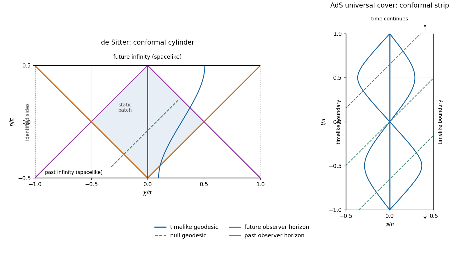
Conformal cylinder and observer horizons of two-dimensional de Sitter spacetime, compared with the timelike boundaries and geodesics of the AdS universal cover
. Details. 
The sides of the de Sitter diagram are identified; its top and bottom are spacelike infinities. The AdS diagram shows a finite window of an infinite time strip, with no identification of top and bottom. Null rays have slope one in both diagrams. The blue curves are timelike geodesics, while the colored de Sitter lines bound the central observer's causal domains.
The geodesics of two-dimensional de Sitter spacetime can be derived directly. Let an overdot denote an affine parameter normalized so that the tangent norm is for timelike, null and spacelike geodesics. The cyclic coordinate gives conserved , and normalization givesWriting reduces this to . For a future-directed timelike geodesic,The spatially comoving curves are geodesics, and every timelike geodesic extends through all , with infinite proper time in both directions. Initially comoving nearby observers have physical separation proportional to , displaying de Sitter's tidal defocusing. Relative separation can initially decrease for other initial velocities; not every pair is monotonically separating.
For a nontrivial null geodesic, and . Hence the conformal infinities at occur at infinite affine parameter, despite their finite values of . For a spacelike geodesic, and . Over a full affine-length period , integrating gives a change . Thus the spacelike geodesics close on the usual cylinder. The special case is the equatorial circle . These closed spacelike curves do not threaten causality.
The geodesics of two-dimensional anti-de Sitter spacetime instead conserve . Their norm equation givesA future timelike geodesic has andIts turning points are . Timelike geodesics oscillate rather than escaping to the spatial boundary. For , the central curve is geodesic. Integrating shows that a full proper-time period advances coordinate time by . They close on the periodically identified hyperboloid but remain complete nonclosed curves on the universal cover. Geodesics leaving reconverge at after proper time , illustrating AdS tidal focusing. A static observer at nonzero fixed is accelerated, not one of these oscillating free trajectories.
For AdS null geodesics, and . They approach either timelike conformal boundary at infinite affine parameter, while the coordinate-time travel from the centre is only . A spacelike geodesic has and connects the two spatial ends with infinite affine length. Both global models are geodesically complete. Reflecting a signal at the AdS conformal boundary is a choice of boundary condition for fields; it is not an automatic continuation of a geodesic at a finite affine endpoint.
For the complete de Sitter observer at , let be the shortest angular distance. An event at can send a signal reaching the observer at a finite future time exactly whenIt can receive a signal sent by the observer at a finite past time exactly when . Equality gives the future and past observer horizons in two-dimensional de Sitter spacetime; their null branches are respectively and on the displayed cylinder. Their intersection is the central static patch, . All complete timelike geodesic observers have analogous horizons by de Sitter symmetry. These are observer-dependent cosmological horizons, not singularities of the global coordinates or Cauchy horizons.
In contrast, the complete central AdS observer can exchange signals with every event at finite : the conformal distance is finite and the observer exists for all . Its static Killing vector has squared norm everywhere. Thus global AdS on its cover has no cosmological event horizon for this observer, although other restricted patches or accelerated observers can have horizons.
The causal predictability distinction is also important. Global de Sitter is globally hyperbolic: constant- circles are Cauchy surfaces. A causal curve is monotone in and satisfies ; if it ended at finite , compactness of the spatial circle would allow an endpoint and extension. Hence an inextendible causal curve crosses every such slice once. AdS on the cover has no closed timelike curves, but it is not globally hyperbolic. For two central events at and , with , their causal diamond contains events at and arbitrarily large , so it is not compact. Initial data alone do not determine field evolution without conditions at the timelike conformal boundaries. de Sitter has spacelike conformal infinities and cosmological observer horizons; covered AdS has timelike conformal infinities and requires boundary data. The distinction between the AdS quadric and its universal cover is also explained in David Tong's general relativity lectures.
Past exam of the mathematics course of the University of Cambridge 2004 iii Paper 55 3 Solution Created 2026-10-03 Updated 2026-10-14
Use units , signature , and the weak-field metric . Define the trace-reversed metric perturbation by , with . In the Lorenz gauge in linearized gravity, , the sign convention of Q2 givesFor completeness, the linearized Ricci tensor in this convention isSubstituting the Lorenz condition and trace reversing gives the stated Einstein tensor. For a stationary source, , so .
Keep the monopole terms of order and the leading term linear in the rotation rate. Since , the latter metric term is of order on the shell. Thus it would disappear from a strictly order- truncation; the requested approximation must retain the leading rotation correction as well. Terms generate metric corrections of order and are neglected. Corrections to four-velocity normalization and the supporting shell stresses affect the omitted higher orders. To retained order,The minus sign in comes from lowering its spatial index; using in its place would reverse the dragging direction.
The scalar Poisson solution regular at the centre and vanishing at spatial infinity is outside the shell and inside. Continuity and the derivative jump verify the density . Also at this order. Undoing trace reversal givesComparing with the scalar parts of the interior line element yields and .
For the mass-current contribution writeEach nonzero angular component is a degree-one spherical harmonic. The supplied Laplacian eigenvalue therefore givesAway from the shell, the two radial solutions are and . Regularity at and decay at infinity select and . Continuity at requires , and integrating the differential equation across the shell givesThus , with . Trace reversal leaves mixed components unchanged, so . The paper writes , giving the frame dragging inside a slowly rotating spherical shellThis dipole matching is valid throughout ; it does not assume the observation point is very close to the centre. The stationary current is divergence-free, so this solution also satisfies the Lorenz gauge. The exterior result is , where the thin shell has , providing a check on the coefficient.
To identify the freely falling frames inside, let be the ordinary spatial rotation by angle . Define the inertial coordinates inside a slowly rotating spherical shell byDifferentiating and dropping , products beyond the retained rotation order, and giveswhich is precisely the interior metric. Thus the retained interior curvature is zero, despite its nontrivial relation to the nonrotating coordinates anchored at infinity. Timelike geodesics in these local inertial coordinates are straight lines , with . In the original coordinates this isunderstood to the same perturbative order. Their coordinate equation is to first rotation order. There is no interior Newtonian acceleration from the constant potential; the velocity-dependent term is the apparent Coriolis term relative to the locally dragged inertial axes.
A freely transported gyroscope at rest in the interior to the retained order has constant spatial direction in the frame, hence its direction in the original axes obeys . Local inertial axes precess in the same sense as the shell, at relative to distant nonrotating axes. This is the interior Lense-Thirring precession. For a weak shell the dragging is only a small fraction of its angular velocity, not perfect corotation. It is compatible with the equivalence principle: rotation relative to distant axes is a comparison between frames, and local flatness at the retained order does not make that comparison vanish. Quadratic rotation terms, which would include centrifugal effects and additional curvature, are outside the requested leading approximation.
Past exam of the mathematics course of the University of Cambridge 2004 iii Paper 55 2 Solution Created 2026-10-03 Updated 2026-10-14
The strong equivalence principle extends universality of free fall to bodies with appreciable gravitational binding energy and requires results of sufficiently local experiments, including gravitational experiments, in freely falling laboratories to be independent of their location and velocity. The Einstein equivalence principle makes the corresponding statement for nongravitational experiments; the weak principle concerns test-body free fall without significant self-gravity. In a locally inertial frame the nongravitational laws take their special-relativistic form, while internal gravitational experiments retain the same local gravitational laws and coupling constants. They are not declared to have no gravity.
In a metric description, one may set and at a point by Riemann normal coordinates, so the Levi-Civita connection vanishes there. This removes a locally uniform external gravitational acceleration, not the Riemann curvature tensor. Tidal effects between separated bodies, or accumulated over a finite-duration experiment, remain. The local limit must control both the laboratory's size and duration. Gravitationally self-bound bodies are included in the strong version, so it is stronger than equality of inertial and passive gravitational mass for ordinary test particles.
A heuristic field-equation argument supplements this principle with further assumptions: gravity is described only by a Lorentzian metric, matter couples universally to it, the affine connection is Levi-Civita, and the leading local field equation is a symmetric covariant equation with at most second metric derivatives and is linear in those second derivatives. Matter obeys stress-energy conservation . Curvature therefore supplies the natural candidates and , with a constant multiple of also allowed. Write the candidate as . The contracted Bianchi identity and metric compatibility giveTo permit varying scalar curvature consistently with matter conservation, take . This gives the Einstein tensor andThe cosmological constant is constant so that its divergence vanishes. These assumptions motivate the usual Einstein equation; the equivalence principle alone does not exclude theories with extra fields or higher curvature terms.
The sign and normalization are fixed by the supplied Newtonian limit. Use signature , the curvature commutator convention of Q1, and the Ricci contractionThis is the contraction for which in the question. In four dimensions, tracing the candidate equation gives , and substituting back givesFor slowly moving pressureless matter, , and . On local scales where the cosmological term is negligible, . Compare this with and the Poisson equation . The Newtonian normalization of the Einstein field equations is thereforeUnits with light speed one are used, as in the paper; for conventional physical stress-energy units the coupling is . If the opposite Ricci/curvature sign convention is adopted, the displayed geometric coupling sign changes accordingly. With the cosmological term retained in the same weak-field calculation, the Newtonian equation becomes , consistent with this sign choice.
Past exam of the mathematics course of the University of Cambridge 2004 iii Paper 55 1 Solution Created 2026-10-03 Updated 2026-10-14
A linear connection on a manifold is a rule for differentiating vector fields which is additive, is -linear in , is real-linear in , and obeys . It extends to covector fields and arbitrary tensor fields by the Leibniz rule and compatibility with contraction. In coordinates,This is the covariant derivative; the affine connection terms correct the changes of the coordinate basis. A symmetric affine connection has zero torsion tensor, , or in a coordinate basis. Symmetry does not imply metric compatibility; no metric is required for this question.
Additivity of each covariant derivative immediately gives additivity of . Expanding the second derivative of a tensor product givesSubtract the expression with exchanged. The two mixed terms cancel, proving that the curvature commutator is a tensor derivation:For a scalar, . Commuting partial derivatives and using the symmetric affine connection gives . Consequently : the commutator is linear over smooth functions, not merely over constant scalars. Write in a local basis. The tensor-product rule gives , showing that its value at a point depends only on at that point. Thus it defines the Riemann curvature tensor byThe antisymmetrized second covariant derivative is itself tensorial in the derivative indices, so this pointwise map transforms as a tensor. The formula or the defining commutator gives , hence with normalized antisymmetrization.
Apply the commutator to the scalar contraction . Its action vanishes, soSince is arbitrary, . Repeated use of the tensor-product rule gives one plus curvature action for an upper index and one minus action for each lower index. In particular,The type notation in the PDF means one contravariant and two covariant indices, not a fractional tensor order.
For the first Bianchi identity, put and . The symmetric Hessian of a scalar field satisfies . Therefore the six third-derivative terms cancel inSubstituting the covector curvature action gives . At a chosen point the gradient of a smooth scalar can be any covector, soThe second form follows from the already proved first-pair antisymmetry.
For the second Bianchi identity, the same third-derivative cancellation can be organized as an operator identity. On vector-valued components set , with . Although a full second covariant derivative includes a term for its lower derivative index, that term cancels on antisymmetrization because the affine connection is symmetric. Thus , where acts by multiplication. Expanding the three nested operator commutators makes all six triple products cancel:Equivalently, the cyclic sum of vanishes. These are the covariant derivative terms on the upper and last lower curvature indices. The two remaining lower indices add . In the cyclic sum these additions cancel in pairs, using and . Hence the Bianchi identities from covariant derivative commutators giveBoth identities here apply to any torsion-free linear affine connection; the second derivation does not require choosing a metric affine connection.
Past exam of the mathematics course of the University of Cambridge 2004 iii Paper 54 4 Solution Created 2026-10-03 Updated 2026-10-14
Compute the honest one-qubit density operators in the computational basis. Writing and , the two quantum state ensembles giveThe equality includes the off-diagonal coherence; comparing only the basis outcome probabilities would not suffice.
The protocol is perfectly hiding against Bob when Alice is honest. Independence of the honest preparations makes his full received density operator . For any POVM , including collective measurements and measurements using ancillas, the Born rule gives the same outcome probabilities . Thus no measurement supplies information about the committed bit.
It is not binding against Alice. Here is an explicit ensemble-steering attack on quantum bit commitment. For each position, Alice prepares the normalized two-qubit pure stateretains and sends . Its partial trace on is the honest common density operator. She sends the halves of independent copies while retaining all the halves, and chooses her bit only at unveiling.
To open one, she makes a projective measurement of each retained qubit in the computational basis. Outcome zero has probability and prepares Bob's state ; outcome one has probability and prepares . She announces that list. It has exactly the honest bit-one distribution, and every declared-state test passes.
To open zero, she instead measures each retained qubit using a three-outcome POVM with effects , whereAll effects are positive. Their diagonal sums are and , and the off-diagonal sum is zero, so . This establishes that the proposed POVM is physically valid.
To verify the conditional states directly, the coefficient matrix of , with Bob's index as the row and Alice's as the column, isA real rank-one effect on Alice's half gives the unnormalized Bob state vector . For the three effects above,Their squared norms are therefore , exactly the honest bit-zero probabilities, and Bob's conditional pure states are the corresponding declared states. Independent measurements on the retained halves produce the honest distribution of the entire list, so even checks on the declared frequencies do not defeat the attack. Every declared-state projector test again succeeds.
Alice can consequently unveil either bit with acceptance probability one, without having chosen it when sending the qubits. This is the Hughston–Jozsa–Wootters theorem mechanism implemented by an explicit measurement, rather than merely an appeal to the general impossibility of perfectly hiding and binding quantum bit commitment.
Past exam of the mathematics course of the University of Cambridge 2004 iii Paper 54 3 Solution Created 2026-10-03 Updated 2026-10-14
Let and choose uniformly from the finite family . All bounds below must hold for every pair of distinct inputs .
A universal hash family, also called universal2, satisfies . A strongly universal hash family satisfiesThus the two outputs are independent and uniform; summing over gives the collision condition. An almost strongly universal hash family permits a larger conditional guessing bound. In the -almost-strongly-universal convention used here,equivalently . Necessarily , with giving strong universality. Stating this normalization matters because the name alone does not specify the allowed forgery probability.
Here is an explicit polynomial almost strongly universal hashing construction and a one-use message authentication protocol. Use a publicly specified finite field , where . Encode a fixed-length -bit message as field elements , padding the final block in a fixed way. Both parties know the length, so this encoding is injective. They share independent uniform secret field elements , requiring shared secret bits. DefineFor every message, the output is uniform because of . For distinct messages and prescribed tags , the condition determines exactly one value of for each . The remaining condition isIts left-hand side has a nonzero coefficient of positive degree, so subtracting the specified constant gives a nonzero polynomial of degree at most . By the root bound for a polynomial, there are at most possible field elements . Consequentlyand this is an -almost-strongly-universal family with , provided . The powers start at one deliberately: a message coefficient at power zero could give a known constant tag shift, allowing a deterministic substitution.
Alice sends the message and its tag over the public channel. Bob accepts only if his independently computed tag agrees. An attacker who has seen no tag guesses one with probability . After seeing a valid pair , an attacker substituting a different message and any chosen tag succeeds with conditional probability at most . This remains true when the choice of depends on the observed pair: the bound is uniform over all those choices. More explicitly, the observed tag leaves uniform because each possible has exactly one compatible secret mask .
For a desired forgery bound , choose . Since and , the substitution bound is at most . The secret requirement isFor a long message this is much shorter than its bits. This is Wegman–Carter authentication: a keyed hash plus a fresh secret one-time pad on the tag. It authenticates the message rather than concealing its contents. Use the key once for the guarantee just established; multiple authenticated messages require fresh masks and a reuse security analysis. Authenticate lengths and sequence identifiers too if variable lengths or replay protection are required.
Past exam of the mathematics course of the University of Cambridge 2004 iii Paper 54 2 Solution Created 2026-10-03 Updated 2026-10-14
There is a necessary distinction between a failure bound averaged over the unknown state, a worst-case bound, and a separate bound for each candidate state. The last interpretation is false: a forger can discard the inputs and always prepare . If the actual state is , every authenticity test passes with probability one. The meaningful uniform statement concerns worst-case failure, or average failure under any fixed prior giving both states positive probability. The PDF does not specify that prior; the argument below gives an explicit bound for either interpretation.
Put . Any unconditional strategy producing output qubits, including ancillas, adaptive measurement in quantum measurements and correlated outputs, is a quantum channel . Its inputs and ideal outputs are the density operatorsThe projective measurements on the different banknotes commute, and their all-pass effect is exactly . Therefore the probability of at least one rejection, conditional on input , isThis remains true for entangled outputs; no independence of their individual test outcomes is assumed.
Use trace distance . The pure-state trace distance and fidelity identity givesFor completeness, two pure-state projectors differ by a matrix with nonzero eigenvalues , which proves this identity. Also the pure-target upper bound on trace distance gives . To see the mixed-state step, write and use convexity of the trace norm followed by the Cauchy-Schwarz inequality:Finally, trace-distance contraction under quantum channels gives . This follows from : the adjoint channel is positive and unital, so its image of any effect is still an effect.
The triangle inequality now yieldsThus the cloning failure bound from trace-distance contraction isand in particular . For positive priors , another Cauchy-Schwarz inequality givesso the average rejection probability satisfiesFor equal priors, one may take ; the same choice is a strict lower bound on worst-case rejection. This proves a quantitative version of the no-cloning theorem for the bank's all-pass test. It concerns an unconditional attempt: heralded success cannot be postselected while omitting failed attempts from the accounting.
Past exam of the mathematics course of the University of Cambridge 2004 iii Paper 54 1 Solution Created 2026-10-03 Updated 2026-10-14
By the Schmidt decomposition theorem, suitable local unitary operations put the normalized pure state into the formIt is entangled precisely when both Schmidt coefficients are nonzero. Put , so for the case of interest. The Pauli operatorssatisfy and in this pure state: fixes both basis terms, and exchanges them.
Choose Alice's two observables as , , and Bob's asThese are valid dichotomic projective measurements. Indeed, and , so ; each observable has outcomes . For the CHSH inequality convention , the quantum value isFor the original pure state, conjugate these four observables by the corresponding local unitary operators. Their outcomes and Pauli correlators are unchanged, and each party still measures only their own qubit. Thus every entangled pure two-qubit state violates CHSH for suitable local measurements, proving Gisin's theorem directly. The CHSH axes for an entangled pure two-qubit state approach a nonviolating configuration continuously as one Schmidt coefficient tends to zero; the strict violation therefore need not be large for weak entanglement.
There are unlisted articles, also show them or only show them.