
Past exam of the mathematics course of the University of Cambridge 2004 iii Paper 5 2 Solution Created 2026-10-03 Updated 2026-10-14
The Brauer morphism retains precisely the fixed group-basis elements under conjugation by :It is unital and surjective because . For multiplicativity, fix . Its coefficient in a product is . Conjugation by permutes these pairs and the summand is constant on each orbit. Nonsingleton orbits have p-divisible size and contribute zero. Singleton pairs have both entries in , so they give exactly the coefficient in . This proves the ring-homomorphism assertion.
Orbit sums form a basis of . A nonfixed orbit sum of is , a proper-subgroup relative trace. Conversely any proper-subgroup trace has zero coefficient on a fixed basis element, since that coefficient is multiplied by in . ThusThere is no assertion that this whole kernel is nilpotent.
Brauer first main theorem bijects the modular blocks of with defect and those of with defect , matching their nonzero Brauer images. Here is a proof with its auxiliary ingredients.
Write , and defineThese are ideals in the indicated commutative algebras, since an invariant multiplier passes through a relative trace. The Brauer morphism and relative trace identityfollows by letting act on . Fixed cosets have representatives in ; projection onto gives equal contributions on each other orbit, whose p-divisible size makes the contribution zero. Thus surjects onto .
To prove the trace criterion for defect groups, choose a p-subgroup of least order with a given block idempotent in . Such a choice exists because a Sylow gives . Write and replace by . If , the kernel formula and trace transitivity give . But is an Artinian local ring, and a finite sum of proper ideals cannot contain its identity. Multiplication by therefore forces for some smaller , a contradiction. Hence .
If is not conjugate into , its action on has no fixed coset and the same orbit argument gives . Every subgroup with nonzero Brauer image of is therefore conjugate into . Its maximal such subgroups are exactly the conjugates of , proving the definition's conjugacy assertion andAmong block idempotents in this ideal, the Brauer image at survives precisely when their defect is .
We also use primitive idempotents under a surjection of commutative Artinian ideals. Decompose the ambient algebras into local factors. The component of an ideal in a local factor is either the whole factor, possessing its identity, or a proper ideal in its nilpotent radical, possessing no nonzero idempotent. A nonzero quotient of a local algebra is local. A surjection of these ideals consequently bijects its surviving primitive idempotents with those of the target. Entire factors may be killed; the whole kernel need not be nilpotent.
Apply this result to . Its surviving primitive idempotents are exactly the modular blocks of with defect . Apply it also to , where the target is identical since and . Its surviving primitive idempotents are exactly the modular blocks of with defect . Matching images in proves Brauer first main theorem, in both directions and with uniqueness.
For the last construction, the intended hypothesis is that is a defect group of the source modular block . Put and use the theorem inside to obtain the corresponding modular block of . The centralizer condition gives , so maps into . Let be the central character of a block, retaining its residue field rather than assuming it equals . The unital compositesends exactly one global block idempotent to one, because their orthogonal idempotent images sum to one in a field. Define to be this unique modular block. This is block induction, independent of the chosen -conjugate of . It needs no containment of in , and its defect may be larger than . With that containment it agrees with the first-main-theorem correspondence.
The printed PDF does not require to be a defect group of . Its literal conditions do not always define the usual induced modular block. For example, over an algebraically closed field of characteristic three, take , as a point stabilizer, and . Then . The ordinary degree-three irreducible of gives a defect-zero modular block on reduction. The two distinct ordinary degree-three irreducibles of give distinct defect-zero modular blocks and . Both restrict to that same character of , with values on its identity, double transpositions and three-cycles.
The standard defect-zero lifting theorem says that these reductions are simple projective modules and their block algebras are full matrix algebras. Thus both module restrictions and contain the same modular block bimodule ; indeed each module restriction is isomorphic to it here. The actual defect of is 1, whose centralizer is , not a subgroup of . The unrelated subgroup cannot select between the two modular blocks. This is block induction requires the block's defect centralizer; the qualified construction above answers the intended request.
Past exam of the mathematics course of the University of Cambridge 2004 iii Paper 5 1 Solution Created 2026-10-03 Updated 2026-10-14
Take finite-dimensional modules over and finite -free lattices over the complete valuation ring, the usual integral modular representation theory convention. If a completion has several local factors, use the factor supporting the modular block. A block of a group algebra is an indecomposable two-sided ideal , where is a primitive central idempotent. The identity decomposes as the sum of orthogonal block idempotents, and for every module. Hence an indecomposable module belongs to exactly when .
A defect group of a block in characteristic is a maximal p-subgroup with . Equivalently, it is minimal with ; the trace criterion for defect groups and conjugacy are proved below. For a complete discrete valuation ring, use the corresponding reduced modular block; modular reduction of block idempotents preserves its defect groups. The equivalent bimodule description says that the module vertices of , with acting by , are conjugates of . This basic characterization follows from the relative-projectivity trace criterion for the bimodule action.
Fix a Sylow subgroup containing . The regular group algebra is the permutation module for , and multiplication by is its block projection. Restriction to a subgroup containing a chosen module vertex retains a summand with that module vertex: a module source at that module vertex is a summand of the module restriction, and the Mackey restriction formula and minimality prevent all the restricted summands from having smaller module vertices. Thus has an indecomposable summand with module vertex .
For a finite p-group , the transitive permutation module is indecomposable: the group algebra of a p-group in characteristic p is local, and this module has a one-dimensional top, incompatible with a sum of two nonzero modules. Its module vertex is , because it is induced from the trivial -module and its Brauer quotient of a module at has the nonzero fixed coset . The fixed-basis rule for this quotient follows by removing nonsingleton orbit sums, which are proper-subgroup traces. It excludes a smaller module vertex. Reduction gives the same statements for permutation lattices. Therefore Krull-Schmidt decomposition identifies the chosen block summand with an entire transitive orbit in .
Choose a point in that orbit whose stabilizer is exactly . Being fixed by every gives . Its full stabilizer isEquality with gives . Conjugating, and using that centralizes , provesThis is defect groups are centralizer-conjugate Sylow intersections.
If is a p-subgroup, then is a p-subgroup for every Sylow , so . It lies in both Sylow factors above. Thus every normal p-subgroup of is contained in .
Finally put , choose , and extend it to a Sylow of . Then and . Apply the proved intersection result to this . Its element belongs to , so is Sylow in too. Hence . The p-core is contained in both factors, whereas normality of in gives the opposite inclusion. Therefore , so is a p-radical subgroup. The centralizer condition on the conjugating element is important for this deduction.
Past exam of the mathematics course of the University of Cambridge 2004 iii Paper 49 3 Solution Created 2026-10-03 Updated 2026-10-14
Use Euclidean worldsheet conventions with . Including a target metric, a Kalb–Ramond field and the dilaton givesThe imaginary coefficient of the antisymmetric term comes from Euclidean continuation; the Lorentzian action has the corresponding real coupling. For constant , the Gauss-Bonnet theorem gives , with Euler characteristic on a connected closed oriented surface. Thus dilaton Euler-characteristic weighting givesAdding one handle multiplies a contribution by , identifying as the string coupling. With canonically normalized external closed-string states, vertices add , giving the string genus expansion .
Before gauge fixing, the Polyakov path integral for inserted string vertex operators is schematicallyThe quotient removes descriptions related by worldsheet diffeomorphisms and Weyl transformations. Gauge fixing has a nontrivial Jacobian, the Faddeev-Popov determinant. Anticommuting vector ghosts and symmetric trace-free antighosts exponentiate this determinant as a local worldsheet ghost action. These worldsheet ghost fields implement the gauge quotient; they are not additional spacetime particles. Their zero modes must be treated separately rather than included in an invertible determinant.
Three kinds of geometry enter the scattering calculation. The worldsheet moduli describe genuinely different conformal shapes that remain after local gauge fixing. Each such shape must be integrated over. The mapping class group consists of orientation-preserving diffeomorphisms modulo those continuously deformable to the identity; it identifies different markings of the same conformal surface, so only one representative of each class is counted. The worldsheet conformal Killing group is the continuous residual conformal symmetry of a chosen surface. It moves insertion positions without changing the geometry and must be divided out, usually by fixing enough vertex positions.
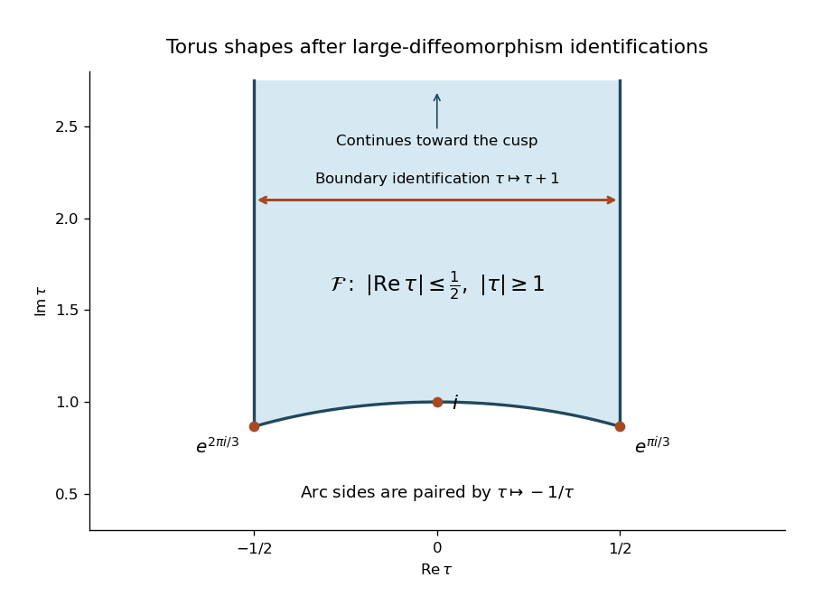
For a torus, write , with . Its shape modulus is , its mapping class group acts through the modular group, and its connected worldsheet conformal Killing group acts by translations. Thus the shape integral runs over the standard fundamental domain of the modular group, while one insertion position can be fixed by translation. On the sphere, three positions can instead be fixed by Möbius transformations; for genus at least two the continuous conformal Killing group is trivial.
Now use the half-normalized worldsheet diffeomorphism ghost operator in the question. A vector field can preserve the representative metric after a compensating Weyl transformation precisely when . The trace of the metric variation sets , leaving the Conformal Killing equationThe kernel of this operator gives the infinitesimal worldsheet conformal Killing group.
For a surviving infinitesimal worldsheet modulus, choose its metric variation orthogonal to all gauge variations. Orthogonality to Weyl transformations requires . On the closed surface, the formal adjoint of the worldsheet conformal Killing operator follows by integration by parts:Orthogonality to every diffeomorphism variation is therefore the adjoint-kernel condition, givingIn a local conformal coordinate these imply and its conjugate: the moduli variations are represented by holomorphic quadratic differentials. Multiplying the definition of by two changes its adjoint by two but changes neither kernel.
For four tachyon vertex operators on the torus, there is one complex shape modulus, four complex insertion positions and one complex translation to remove. The worldsheet integration count after conformal gauge fixing is thereforeFix the fourth insertion at . A schematic gauge-fixed expression isHere the antighost pair supplies the modulus measure, and the ghost pair at the fixed vertex absorbs the translation zero modes. The three unfixed positions and are the four complex integrations. The punctured Riemann surface moduli dimension gives the same result, . Target-spacetime zero-mode integrals producing momentum conservation are separate from this requested count of worldsheet integrations.
Past exam of the mathematics course of the University of Cambridge 2004 iii Paper 49 2 Solution Created 2026-10-03 Updated 2026-10-14
The string sigma model in a spacetime metric is the Polyakov actionTake conformal gauge , and choose spatial period for the closed string. Substitution of the plane-wave metric givesThe stipulated light-cone gauge in string theory sets and . Its longitudinal term is a total time derivative. The transverse string sigma model in an isotropic plane wave is thereforeThe resulting Euler-Lagrange equations are the massive wave equationsThese conventions fix the mass term directly from . More generally would replace by , with for this spatial period.
Use the real orthonormal Fourier basisFor the plane-wave string mode frequencies, let and . The complete real mode expansion for nonzero frequencies isEvery term obeys the wave equation and is periodic. Orthonormality and completeness let its coefficients match arbitrary appropriate initial position and velocity data. For , replace the zero-mode bracket by ; the zero mode becomes a free particle rather than an oscillator.
The canonical momentum density is . The transverse Hamiltonian isWrite and . Since and , substitution gives the plane-wave string mode HamiltonianThis is a collection of independent harmonic oscillators. The last equality follows by substituting the sine-and-cosine time dependence; each oscillator energy is constant.
For canonical quantization of each nonzero-frequency mode, putThen . Opposite travelling-wave oscillator combinations give the equivalent formFor , the formal zero-point energy is . At , replace the zero-mode occupation term by . The zero-point expression is divergent and needs a regulator or a specified normal ordering convention; no mass-independent intercept has been assumed.
The remaining Virasoro constraints determine the longitudinal coordinate:Periodicity of imposes , the closed-string level matching condition. Labelling the travelling oscillators by their opposite worldsheet momenta gives . The light-cone energy equals , consistent with the positive mass term in the Hamiltonian.
This is the classical reduction in the specified background. As a full quantum background with constant dilaton and no Kalb–Ramond field, this metric has and fails the lowest-order sigma-model beta function equation when ; additional background fields would be required for quantum Weyl invariance.
Past exam of the mathematics course of the University of Cambridge 2004 iii Paper 49 1 Solution Created 2026-10-03 Updated 2026-10-14
Use a mostly-plus target metric tensor and the standard open-string mode expansion convention . The integer string oscillator level is , whose eigenvalues are nonnegative integers. Then , so the string mass-shell condition givesThe ground state is a tachyon, and the level-one state is massless. The physical string state conditions in old covariant string quantization areOnly the positive-mode Virasoro constraints annihilate a ket; their negative-mode partners annihilate the corresponding bra. Imposing both signs on every ket would contradict the nonzero Virasoro central extension.
The central charge comes from normal ordering the quadratic oscillator expressions. Classically their Poisson brackets have no central term. Quantum mechanically, moving annihilation operators through creation operators produces double contractions. From the oscillator commutator one obtains , which gives the noncentral part .
The coefficient is fixed by the free-boson Virasoro central term. On a formal zero-momentum vacuum, for ,The two contraction pairings giveHere ; the time coordinate contributes one, just as each spatial coordinate does. Comparing with the Virasoro algebra provesThis counts covariant target coordinates. It is distinct from the physical transverse polarizations. Including the central charge of reparameterization ghosts gives ; cancellation of the worldsheet Weyl anomaly gives the usual critical dimension of the bosonic string .
A general level-one state isThe zero-mode constraint requires . Since , the remaining nontrivial positive-mode constraint is ; all with act trivially at this level. Thus the polarization vector is transverse to a nonzero null momentum.
There is also a null string state . It is physical when and orthogonal to every physical polarization. The null-state quotient of a string therefore identifiesChoose . Transversality sets , and the null-state identification removes this common component. The remaining spatial components have positive norm. Hence the physical level-one states form a massless vector with polarizations, or 24 at the critical dimension. The removed component is gauge redundancy. States violating the constraints, including independent timelike negative-norm polarizations, are unphysical; physical null states are removed by the quotient rather than counted as additional particles.
Past exam of the mathematics course of the University of Cambridge 2004 iii Paper 48 4 Solution Created 2026-10-03 Updated 2026-10-14
Put and neglect electron and final-quark masses compared with . First fix a final color charge; its multiplicity will be restored for the inclusive rate. The photon-exchange scattering amplitude is, up to an overall phase,Averaging over the two spins of each incident particle and summing final spins givesBy the gamma matrix trace identities, the first trace is , and likewise for the second. Contracting the two tensors cancels the terms proportional to , givingIn the centre-of-mass frame all four energies are . The first pair of scalar products equals each, and the second pair equals each. Hence .
For clarity, the printed flux hint has a factor-of-four inconsistency: when , the prefactor multiplying the spin-averaged amplitude is , not . Alternatively, is correct if . Use this massless two-body scattering flux normalization, keeping the spin average separate.
To obtain the two-body Lorentz-invariant phase space directly, integrate the momentum-conserving spatial delta function, leaving . The remaining radial integral is , so . The relativistic scattering cross-section is consequentlySince , the integrated electron-positron annihilation into a quark pair result, for this fixed color, isThe first two printed formulas are thus color-stripped. Distinct final colors are orthogonal states and must be summed, producing . At leading order each accessible quark flavor contributes independently. Away from thresholds and narrow resonances, quark-hadron duality relates the inclusive parton rate to the observed inclusive electron-positron annihilation into hadrons, givingThis formula concerns the photon channel, assumes is large compared with the relevant quark masses and the strong-interaction scale, and does not include Z boson exchange.
Beyond leading order, an exactly exclusive pair of colored quarks is not an observable asymptotic state because of confinement and hadronization. Moreover its virtual corrections have infrared divergences; real soft or collinear gluon emission cannot be excluded if a finite rate is wanted. The inclusive sum includes both the corrected two-parton channel and channels such as , with their degenerate soft and collinear limits. Real and virtual infrared divergences then cancel for an infrared-safe observable. A specified jet observable can also be meaningful if it defines an infrared-safe observable; a bare two-quark final state is not.
A convenient inclusive calculation uses the optical theorem. For the electromagnetic hadronic current , defineThe hadronic electromagnetic-current spectral density is obtained from its discontinuity. In this convention the hadronic R ratio is , where at this order. Cutting the forward amplitude sums all allowed hadronic intermediate states, so perturbative Quantum chromodynamics applied to this inclusive quantity implements the required sum of real and virtual contributions.
Finally, write , , , and . The given truncated correction isDifferentiate with respect to , using the stated one-loop beta function and . The derivative of cancels the explicit logarithmic derivative at order . Keeping the residual derivative of the truncated expression givesThus the principle of minimal sensitivity, applied to this expression with nonzero coupling and , selects the one-loop stationary scale for the hadronic annihilation correctionThis is a prescription based on the residual order- scale dependence of an order- approximation. At strictly order , the derivative already vanishes for every renormalization scale; the prescription does not assert exact scale dependence of the observable. It is useful only while the selected running coupling remains perturbative. If or , the stated derivative imposes no unique scale.
Past exam of the mathematics course of the University of Cambridge 2004 iii Paper 48 3 Solution Created 2026-10-03 Updated 2026-10-14
Start with the Dirac equation . The equation for the Dirac adjoint is . Transpose it and multiply by the charge-conjugation matrix C to obtainFor this to be the original Dirac equation multiplied by minus one, the necessary matrix identity isUsing , the charge conjugation of the Dirac adjoint follows directly:The final step uses and .
Let , , and . For anticommuting fields, or normal-ordered operator bilinears, the minus sign in the transformed Dirac adjoint cancels the minus sign from interchanging the two fields. The charge conjugation of fermion bilinears is thereforeThe matrix identity just proved gives . Also , obtained by transposing its four gamma matrices and reversing their order. Henceso and , where . Since the external vector V is odd under charge conjugation, becomes and is generally not invariant.
For parity symmetry in quantum field theory, write . The given spinor transformation gives , , and , with arguments evaluated at the reflected point. The contracted interaction again becomes . Each of parity and charge conjugation interchanges the two chiral contractions; applying both restores . This particular neutral current interaction is CP invariant, although neither P nor C is separately a symmetry. This conclusion uses the stipulated C-odd vector transformation; it is not a claim that all interactions of the Standard Model preserve CP symmetry.
For time reversal of a Dirac field, the gamma matrix adjoint and transpose identities giveWith , anticommutation of with every gamma matrix yieldsEquivalently, . Since time reversal is an antiunitary operator, the factor i in must also be conjugated. ThusUsing the stated transformations of the field and its Dirac adjoint, the transformed bilinear consequently isThe external vector has the same component signs. Their contraction is unchanged, proving time reversal of a real neutral chiral vector interaction. A real coupling is understood; an antiunitary operator also conjugates coefficients, and relative complex weak phases need not satisfy this invariance.
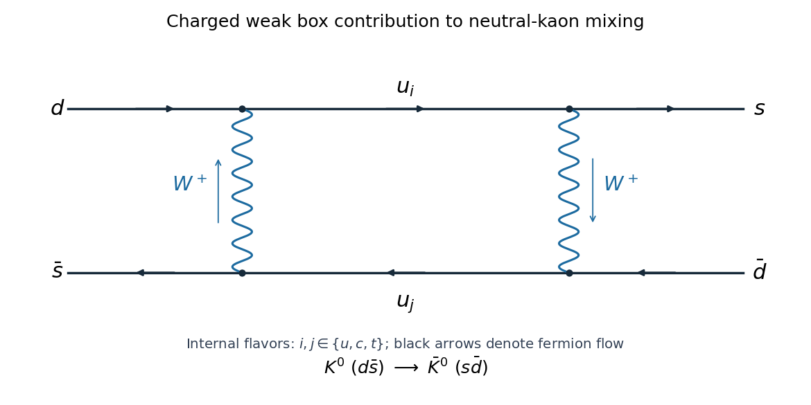
A charged weak box contribution to kaon mixing is shown below. The incoming and outgoing connect through two charged W bosons and two internal up-type quarks. The black arrows are fermion flow, so the lower line's arrows oppose the momentum of the corresponding antiquark. The blue arrows specify the direction of positive charge carried by the charged propagators. Each vertex is a charged weak current vertex, with the appropriate CKM matrix element; the internal flavors are summed over .
Use precisely the printed exchange-positive CP convention for neutral kaon mixing. In the flavor basis, CP symmetry acts by . Write the restricted effective matrix asThen , so CP invariance of this mixing operator is exactly . Therefore CP noninvariance in this neutral-kaon mixing block means . Violation elsewhere in a larger Hamiltonian would not, by itself, prove an inequality for this particular block.
For neutral-kaon mass matrix diagonalization, choose correlated roots , , and eigenvalues . The vectors and are the corresponding eigenvectors, as direct multiplication verifies. Taking orthonormal flavor states and writing the printed CP eigenstates as and , one findswhere the kaon CP mixing parameter isOverall phases have been absorbed. The kaon mixing square-root branch convention must be chosen continuously so that in the CP-conserving limit for the eigenstate labeled plus. These formulas are exact in the nondegenerate case with ; the requested small admixtures follow if . Smallness is an additional weak-CP-violation assumption, not a consequence of alone. A Hermitian mass operator has ; the same algebra also applies to the effective non-Hermitian operator that includes decays, where the two eigenstates need not be orthogonal. At a fully degenerate , a CP eigenbasis can simply be chosen.
Past exam of the mathematics course of the University of Cambridge 2004 iii Paper 48 2 Solution Created 2026-10-03 Updated 2026-10-14
The derivative convention uses hypercharge Y with . For each lepton family , the left-handed fields form an SU(2) doublet , with . Their weak isospin values are and their electric charges are . The right-handed charged lepton is an SU(2) singlet, with , and charge . The minimal model used here has no right-handed neutrino. A sterile right-handed neutrino, if added as a singlet with , would have no charged weak current interaction. Antiparticles carry the conjugate representations and opposite electric charges.
Expanding supplies . The off-diagonal entries of are and . With the chiral projector , one has . Thus the two W boson interactions areFor quarks, separate rotations diagonalize the up-type and down-type mass terms. If their left-handed rotations are and , the charged interaction contains the CKM matrix :There is an implicit sum over color charge. This quark mixing permits transitions between different families, rather than just the paired fields in a single doublet.
Let and . At momenta much smaller than , neglect derivatives in the heavy W boson equation. Its mass and source terms can be completed to a square:This explicitly performs integrating out a charged vector boson. The resulting Fermi interaction isThe omitted terms contain derivatives and are relatively suppressed by momentum squared divided by .
For the leptonic pion decay, Lorentz covariance restricts a vacuum-to-spin-zero current matrix element to a constant times . In the rest frame, rotations eliminate the spatial components. Under parity, the temporal vector current is even, whereas the vacuum is even and the pion is odd, so its temporal matrix element equals its negative and vanishes. The temporal axial current is odd and is allowed. This proves the vacuum-to-pseudoscalar current selection rule, rather than merely assuming an axial current. Define the pion decay constant byThen the vector-minus-axial charged weak current has matrix element , up to an irrelevant overall phase convention. Consequently the scattering amplitude for the decay can be writtenUse , the momentum-space Dirac equation , and for a massless neutrino. Since , the neutrino contribution vanishes, leavingThe fermion spin sum is, using the supplied gamma matrix trace identities,Here , , and . The mass term in the trace vanishes; anticommuting reduces the remaining trace to twice . It follows thatUsing two-body decay phase space, with final momentum magnitude , gives the leptonic pseudoscalar decay widthThus the requested factor is already present in the squared amplitude, and the phase space supplies one more threshold factor.
The physical explanation is helicity suppression. In the pion rest frame the two momenta are opposite. The massless antineutrino has positive helicity; zero total angular momentum would require the electron to have positive helicity too. The charged weak current instead creates a left-chiral electron, whose helicity is negative when its mass vanishes. A nonzero electron mass admits the required opposite helicity with an amplitude proportional to . The decay amplitude vanishes for , and the rate is suppressed by .
Past exam of the mathematics course of the University of Cambridge 2004 iii Paper 48 1 Solution Created 2026-10-03 Updated 2026-10-14
Work with canonically normalized real components of the scalar field; a complex representation can first be written in terms of its real and imaginary components. At a vacuum expectation value , expansion of the scalar potential givesThe linear term vanishes by stationarity. Thus the scalar mass matrix is the Hessian matrix of the scalar potential. Invariance under each Lie algebra generator gives the identity . Differentiating this identity with respect to and evaluating at the stationary point removes the term containing , leavingThe kernel of the map is precisely the Lie algebra of the stabilizer subgroup H. Consequently its restriction to a complementary space of broken Lie algebra generators is injective: a linear combination that annihilates would belong both to the stabilizer algebra and its complement, and hence would vanish. There are therefore independent Goldstone directions in the scalar mass matrix, tangent to the vacuum manifold. There are symmetry-protected massless scalars.
This Goldstone theorem guarantees at least that many zero quadratic masses. The claim that these are all the massless scalars additionally requires nonzero curvature transverse to the vacuum orbit. For example, , with , has an ordinary spherical vacuum manifold but its entire Hessian matrix vanishes there. These accidental massless radial modes beyond Goldstone modes are not excluded by the hypotheses. For the indicated orthogonal group breaking, the protected number is
For the Higgs doublet, put and wherever . If , thenThis explicitly exhibits the three angular coordinates as an SU(2) transformation of a real radial field. In particular, the polar coordinates for the electroweak Higgs doublet can locally be chosen in the formAt the vacuum the three variations generated by , , and acting on are independent over the reals. They span the three broken directions; the remaining generator annihilates the vacuum. This proves that the exponential supplies local angular coordinates. An inverse local gauge transformation, applied also to the gauge fields, removes these three fields in unitary gauge. They supply the longitudinal polarizations of the massive W bosons and Z boson through the Higgs mechanism. The parameterization is local about a nonzero vacuum, rather than a coordinate system through every possible zero of the Higgs doublet.
Use the metric and define the charged W bosons and neutral gauge fields bywhere , , and . Direct substitution into the gauge-covariant kinetic term givesand henceThe electroweak doublet gauge-boson mass matrix in the basis isIts normalized zero direction is and its massive direction is . Thus the scalar-vector terms in physical fields arewith the tree-level electroweak gauge-boson massesThese are also charge eigenstates. The unbroken U(1) gauge symmetry has generator ; on the Higgs doublet, . Since , the combinations have charges , while Z, the photon, and H are neutral. The photon disappears from the displayed scalar-vector terms because . The photon is massless and has no direct tree-level coupling to the remaining radial scalar in this sector. This does not remove its interactions with charged W bosons, or exclude a scalar-to-photon interaction generated by loops.
Finally, retain the printed normalization of the Higgs field potential:The kinetic term is , so the Higgs radial mass for a half-normalized quartic potential is . The extra factor of two familiar from a potential with prefactor , rather than , does not apply here.
Past exam of the mathematics course of the University of Cambridge 2004 iii Paper 47 4 Solution Created 2026-10-03 Updated 2026-10-14
Choose a definite matrix convention: , , and . Matter transforms as , so gauge covariance requires . Applying both sides to a test field yields the Yang-Mills gauge transformationDefine the Yang-Mills field strength by :Conjugating the gauge covariant derivative commutator proves : unlike the connection, the gauge field strength has no inhomogeneous derivative term. The trace normalization supplies an invariant color metric; its Lie algebra structure constants with all indices lowered are antisymmetric.
For and , expand the finite transformations:In components this isA convention using the opposite matter transformation or gauge covariant derivative sign changes these signs consistently. The formulas above all follow from the explicitly chosen .
Gauge reduction and the determinant. A direct integral integrates repeatedly over gauge-equivalent configurations. The gauge group volume is infinite, and the ungauge-fixed quadratic operator has longitudinal zero directions, so it has no ordinary inverse quantum field theory propagator. Gauge-invariant observables require dividing out this redundancy rather than treating it as an ordinary physical fluctuation.
The finite-dimensional change-of-variables identity underlying gauge fixing is precise. Suppose a condition has one solution in the group-coordinate patch and its derivative matrix at the solution is nonsingular. ThenFor several isolated solutions it instead counts those solutions. On the slice, the Jacobian determinant can be factored into the reciprocal of the orbit integral of the delta function. An invariant measure and invariant integrand then allow the group volume to factor out. In the functional version, group coordinates carry Haar measure and the corresponding operator determinant replaces the matrix determinant.
For example, choose the Lorenz gauge . Its variation is . Hence on the gauge slice the Faddeev-Popov operator and Faddeev-Popov determinant areIts extension along each local gauge orbit yields the Faddeev-Popov gauge-orbit identityFor an unoriented finite-dimensional real integral the absolute determinant is required. In a perturbative gauge patch, its sign or phase is fixed and the constant convention is absorbed in normalization. Residual zero modes must be removed by boundary conditions or separate treatment. Multiple intersections, the Gribov ambiguity, prevent interpreting this as a globally unique gauge slice without additional work.
Insert the identity, change variables along the orbit using invariance of the action and measure, and divide out the common gauge group volume. Averaging with Gaussian weight produces the covariant gauge-fixed functionalThe added term makes the quadratic gauge-field operator invertible after the stated residual-mode treatment.
Ghost representation. For a finite matrix , the Grassmann Gaussian integral over independent anticommuting variables is proportional to its determinant:The constant is independent of and depends on ordering and factors of . The functional counterpart introduces Faddeev-Popov ghost fields and antighost fields , withIntegration by parts writes its density as , displaying a kinetic term and a gauge-field/ghost interaction. These are Grassmann-valued fields with scalar Lorentz transformation law. They represent the orbit Jacobian determinant; their closed loops carry the fermionic minus sign, and they are not physical asymptotic particles. In the abelian case , the determinant is gauge-field independent and the ghosts decouple. Nonabelian ghosts interact and are necessary for the consistent cancellation of unphysical gauge contributions.
Physical-state reduction. Let be the Hermitian BRST charge. Its key algebraic property is BRST nilpotence, , and the gauge-fixed dynamics preserves it. Physical states are its BRST cohomology at ghost number zero:Here has ghost number . BRST nilpotence ensures that exact vectors lie in the kernel, so the quotient is defined. Because is Hermitian, an exact vector is orthogonal to every closed vector, , and exact vectors are null, . They therefore represent no independent physical state. Commutation of with the Hamiltonian preserves these classes under time evolution.
The covariant gauge/ghost space before reduction has an indefinite inner product. This is essential: a Hermitian nilpotent BRST charge requires an indefinite auxiliary space if it is nonzero. On an ordinary positive-definite Hilbert space the same norm identity would force . Positivity of the resulting physical space uses the gauge-theory structure in addition to the abstract BRST nilpotence identities.
For a nonzero on-shell photon momentum, the one-particle conclusion isThe second relation preserves the first because . In four dimensions the transverse kernel has dimension three, and quotienting by its null longitudinal direction leaves two physical photon polarizations. This is the positive one-particle BRST cohomology of the photon sector.
Past exam of the mathematics course of the University of Cambridge 2004 iii Paper 47 3 Solution Created 2026-10-03 Updated 2026-10-14
Use the mostly-minus Minkowski metric, quantum field theory propagator and dimensionally continued interaction , with . Take all four external momenta incoming, so , and set , , .
The three one-loop one-particle-irreducible Feynman diagrams are the bubble graphs with external pairings , and . Their external quantum field theory propagators are omitted by amputation. Each Feynman diagram has symmetry factor from exchanging the two internal lines; the fixed external labels are already accounted for by the three distinct channels.
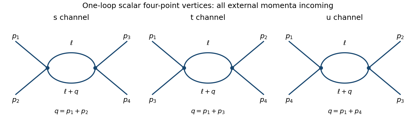


For a channel carrying momentum , its amplitude isThe signs in the last equality follow from the two vertices and two quantum field theory propagators. Apply the Feynman parameter identityAfter shifting the loop momentum, the denominator is , with . For positive Euclidean , Wick rotation and the Schwinger representation giveAnalytic continuation to physical momenta keeps the prescription . Thus dimensional regularization evaluates the channel asUse and expand the other factors. The minimal-subtraction scalar four-point bubble channels result through the finite part isThe parameter integral is left unevaluated, as requested. The three channel contributions are . Their pole is momentum independent and is cancelled by the four-point counterterm , withAfter pure minimal subtraction scheme subtraction, the complete vertex through one loop is the tree vertex plusHere the limit has been taken. The modified minimal subtraction scheme would also absorb ; it is not identical to the specified pure MS finite part.
The bare coupling is scale independent and satisfiesWriting and differentiating at fixed givesAt order , the finite coefficient is , so the one-loop quartic scalar beta function isThe factor two relative to the pole residue follows from using . With the residue doubles, but the four-dimensional beta function is unchanged.
For pure nonabelian gauge theory, the corresponding pure Yang-Mills one-loop beta function has the opposite sign:Gauge-boson self-interactions and the gauge-consistency ghost contributions give antiscreening. For a compact nonabelian simple factor , the coupling decreases at high energy: asymptotic freedom. In contrast, positive scalar increases toward the ultraviolet. Its one-loop extrapolation has a Landau pole, indicating breakdown of weak-coupling perturbation theory, not a proof by itself of nonperturbative triviality. Ultraviolet poles should be extracted at infrared-safe mass or nonexceptional kinematics; a scaleless massless zero-momentum integral cannot be used to read off this ultraviolet counterterm without separating its infrared behavior.
Past exam of the mathematics course of the University of Cambridge 2004 iii Paper 47 1 Solution Created 2026-10-03 Updated 2026-10-14
Use a Minkowski external source term , where is the integration variable, and normalize the vacuum functional:The usual vacuum boundary prescription is implicit. This is the logarithmic convention for the connected generating functional. It makes the given quadratic expression consistent with . Another common convention is , with ; mixing the two conventions would change the factors of below.
Functional derivative generates the full and connected correlation functions:These are time-ordered products in the vacuum, and by the stated assumption. Differentiating four times partitions the four insertions into connected blocks. All partitions with a singleton vanish, leavingThe shorthand arguments stand for spacetime points; this is a functional cumulant identity, not an assumption of a free field.
To construct the quantum effective action, define the source-dependent classical fieldLocally invert this relation to obtain , assuming the response integral kernel is invertible with the chosen regulator and boundary prescription. Take its Legendre transformThe chain-rule terms proportional to cancel, so . A field-independent constant is fixed separately and is immaterial to the vertices. At zero external source the classical field is zero, and there is no linear term.
For the two-point vertex, differentiate the classical field once. If , thenThe vertex coefficients in this problem are derivatives of , not of alone. ThereforeFor the three-point vertex, the derivative of the connected two-point integral kernel at a general external source isCombine this with and differentiate the inverse identity, . This gives the logarithmic-source inverse-kernel vertices relationAll kernels here are finally evaluated at zero external source. The connected three-point function is amputated by its three inverse quantum field theory propagators.
For the specified quadratic , the external source response is , hence . Substitution in the transform givesFor the standard free quantum field theory propagator , this is the usual quadratic free action, up to the vacuum prescription. The generating functional is Gaussian, so connected functions beyond second order vanish and there are no interaction vertices or nontrivial scattering amplitudes. Full higher even-point functions can still be nonzero: they are products of two-point functions, as the four-point formula shows.
Past exam of the mathematics course of the University of Cambridge 2004 iii Paper 46 3 Solution Created 2026-10-03 Updated 2026-10-14
The partition function sums the Boltzmann weights of all statistical configurations. For discrete states of energy , ; for a regulated scalar field it is a functional integral, . It normalizes probabilities and generates thermodynamic averages. Its Helmholtz free energy isA quantum version uses . In the following identification, is a constrained free-energy density, so its units match those of a Hamiltonian density rather than a total extensive energy.
Fix a microscopic cutoff . Split the field into retained modes with momenta below and eliminated modes between and . Define the Wilsonian coarse-grained statistical Hamiltonian exactly byIts coefficients and additive constant depend on so that integrating the retained modes gives precisely the original . With sources and observables carried along, the same construction preserves long-wavelength responses. Thus changing this intermediate ultraviolet cutoff is a change of description, not a change of the physical system. It is advantageous because one can integrate out fluctuations irrelevant to the observable length scale, organize a local gradient expansion, and use renormalization-group flow toward simpler universal fixed-point descriptions. Exact invariance retains all generated operators; truncating them is an approximation.
The quadratic gradient coefficient generally becomes , not a constant. Field renormalization sets a chosen kinetic normalization, for example when this makes the gradient coefficient one in the energy convention. Sources and observables must be transformed inversely so that their physical meaning is preserved. Under rescaled coordinates , the critical field scaling isIts anomalous part is the anomalous dimension; it gives and the conjugate-field exponent . Different conventions for the wave-function factor require corresponding changes in its logarithmic derivative. A fixed physical magnetization must not be confused with a cutoff-dependent dimensionless renormalized field.
To justify the zero-cutoff identification of constrained free energy, work first in a finite periodic volume . Define the physical spatial mean and constrain that mean in the microscopic integral:Retain the constant mode while eliminating every nonzero mode. When is below the smallest nonzero box momentum, the remaining energy is . Consequently with a consistently fixed, possibly field-independent measure normalization. This provesFor a uniform field, is the Hamiltonian density in the question. The statement assumes that the physical zero mode is retained, all other modes are integrated exactly, field-rescaling factors are undone, and density and additive-normalization conventions agree. Taking the cutoff limit in the finite box before its thermodynamic limit makes this derivation unambiguous. With an applied uniform source, up to the same measure convention; its large-volume saddle minimizes .
The Landau approximation further assumes that this potential can be approximated by a regular local polynomial on the homogeneous branches, and that the remaining fluctuations are negligible for the observables sought. It is not an assertion that an exact zero-cutoff free energy is the bare polynomial. In a coexistence region the exact constrained density can be convexified by domains, while a nonconvex Landau branch potential describes local phases and their metastability.
For the breakdown criterion use a short-range scalar theory with positive quadratic gradient stiffness. At the Gaussian fixed point, invariance of gives field dimension . A coupling multiplying therefore has engineering scaling exponentIt is irrelevant only above its upper critical dimension. For the ordinary critical point the leading stabilizing interaction is quartic, while at a tricritical point the renormalized quartic term is tuned away and the leading interaction is sextic. ThereforeOne can also see the failure through the Ginzburg criterion. Long-wavelength fluctuations averaged over a correlation volume obey , up to temperature and stiffness factors. The quartic saddle has , giving a fluctuation/mean-square ratio proportional to . The tricritical sextic saddle has , giving a ratio proportional to . Both ratios grow without bound below their respective critical dimension, invalidating the fluctuation-free Landau exponents sufficiently close to a transition.
At equality the ratios are marginal, not power-law divergent. The loop expansion resolves this boundary: the quartic vertex correction contains , logarithmic at ; the sextic vertex correction contains a two-loop three-propagator integral whose overall degree is , logarithmic at . Marginal running therefore generally adds logarithmic corrections at these dimensions. Below them, where the corresponding transition exists, interactions control the long-distance critical behavior. Above them, leading thermodynamic powers are mean-field, although stabilizing dangerously irrelevant couplings explain why naive hyperscaling need not hold.
There are unlisted articles, also show them or only show them.