
Past exam of the mathematics course of the University of Cambridge 2004 iii Paper 46 2 a Created 2026-10-03 Updated 2026-10-14
Past exam of the mathematics course of the University of Cambridge 2004 iii Paper 45 4 Solution Created 2026-10-03 Updated 2026-10-14
In the finite-dimensional complex semisimple Lie algebra setting, the rank of a semisimple Lie algebra is the dimension of a Cartan subalgebra , equivalently the number of independent commuting Cartan generators. For a compact real algebra, use its complexification and the corresponding maximal torus. Simultaneously diagonalizing the commuting adjoint actions of gives the root-space decompositionThe nonzero linear functionals for which this space is nonzero are the roots of a root system. An invariant inner product identifies them with vectors in a real Euclidean root space. These are the usual semisimple assumptions behind the rank and root language here.
The displayed generators form an sl2 triple. Start with a nonzero lowest-weight element and define . The Jacobi identity givesInduction starting with consequently gives the finite sl2 lowest-weight ladder weightsNow commute the lowering equation with and again use the Jacobi identity:The left side is . Whenever , coefficient comparison givesThe initial condition is , meaning ; directly , so . Summing the recurrence from to yieldsIn fact the vector identity follows inductively from the same Jacobi identity without needing a separately assumed lowering coefficient.
If is the last nonzero element and , apply to this zero next element. The lowering identity givesso , a nonnegative integer. The nonzero endpoint is necessary. Literally allowing would make the printed conclusion false: take in the adjoint representation of . Then , , , . Choosing gives a vanishing next bracket but not . The intended endpoint is the first terminating bracket after the nonzero ladder.
For the plus-sign nested commutators, use , and . The cross relation gives , while . Thus the lowest-weight label is . If the -fold raised element is nonzero and the -fold element vanishes, the preceding endpoint argument gives and henceFor the minus-sign ladder, use the sl2 triple , , and start at . Its lowest-weight equation is again , and its lowering bracket vanishes by the cross relation. The same argument proves exactly the same result, including the endpoint assumption that is explicit in the nested-commutator question.
For arbitrary roots of a root system , choose the normalized sl2 subalgebra associated with a root , whose generators obey and . The coroot normalization givesThe normalization has a concrete construction. Use the nondegenerate Killing form , and define by . Invariance makes root spaces orthogonal unless their roots sum to zero, so there exist and with . Invariance then gives , hence . With , take , and . Their brackets have the required normalization and . Let be a nonzero root vector with weight . Repeatedly apply until reaching a last nonzero vector . Its weight is . This process terminates because different weights are linearly independent and the Lie algebra is finite-dimensional. Starting at , repeatedly raise; this also terminates for the same reason. The proven lowest-weight endpoint formula says for a nonnegative integer . ThereforeThis proves integrality of Cartan integers directly from the finite ladder, rather than assuming the crystallographic axiom.
Finally use the indices actually printed in the PDF: , , , . The converted TeX has corrupted these indices. The prescribed bracket is that of trace-free matrix units. The sum of the diagonal generators is zero, leaving two independent diagonal elements, and their pair brackets giveFor example , and the analogous second pair gives . The cross raising-lowering brackets vanish. A diagonal with entries has . Thus acts on with weights , and acts on them with weights . The negative generators have the opposite weights. In the question's index ordering,This is the Cartan matrix of the A2 root system, and the Lie algebra generated by these matrix units has rank two. As an additional bracket check, whereas , so the nested ladder has and indeed . The negative ladder likewise terminates after one nonzero bracket.
Past exam of the mathematics course of the University of Cambridge 2004 iii Paper 45 3 Solution Created 2026-10-03 Updated 2026-10-14
In the two-body centre-of-mass frame, spatial reflection reverses the relative coordinate of a quark-antiquark pair. Its orbital state of angular momentum has orbital parity , as follows from . Opposite constituent intrinsic parities multiply to minus one. Thus the meson parity and charge conjugation rules begin withTo obtain charge conjugation, consider a self-conjugate flavor state and write its spin-orbital wavefunction using ordered creation operators . Charge conjugation interchanges the quark and antiquark operators. Reordering them back to quark-first order produces a fermionic sign minus one. Interchanging the two spin- labels has eigenvalue in the spin singlet state () and in the spin triplet (), namely . Reversing the relative momentum contributes . ThereforeReciprocal phases for the two conjugate creation operators cancel, so the result is independent of that convention. This applies to a state that is mapped to itself by charge conjugation, not to every electrically neutral flavor state. For example a neutral meson with unequal quark and antiquark flavors can be exchanged with a different antimeson. Charged states have no individual eigenvalue.
Restrict flavor to the isospin doublet. Its product with the conjugate doublet decomposes as . Convenient normalized flavor states, with irrelevant overall phase choices, areOrbital excitation normally costs energy, so the simplest low-lying quark model states have . Coupling the two constituent spins gives or , and then . The isotriplet with is the pion triplet, while the isotriplet with is the rho meson triplet. The isosinglet with is the nonstrange component of the omega meson. Their quantum numbers areThe charged pions have and the charged rho mesons have ; charge conjugation exchanges the positive and negative members. The same tensor product also allows an , pseudoscalar state, so symmetry alone does not assert that only the listed mesons exist or predict their masses. The physical isosinglet spectrum involves further dynamics and, when strange flavor is included, mixing.
For a vector-meson decay to two spinless pions, conservation of angular momentum forces their relative orbital value to be . Their combined parity is , and the neutral charge combination has , matching both and . Thus and alone do not distinguish these two decays. The decisive restriction is isospin together with Bose statistics.
Two isotriplet pions have , or total . Under exchange the isospin- state has sign : the highest state and its lowered partners are symmetric, the highest combination is antisymmetric, and the singlet is symmetric. The orbital state is antisymmetric. Since pions are spin-zero bosons, their total state must be symmetric, requiring the antisymmetric isospin sector . This allows but excludes an isospin-conserving amplitude.
There is no analogous obstruction for three pions. In a Cartesian isospin basis , their totally antisymmetric combination is an state. It can multiply a totally antisymmetric momentum amplitude proportional in the rest frame toMomentum conservation makes this amplitude change sign under every exchange of two pion labels. The product of the flavor and momentum factors therefore obeys Bose statistics. The cross product supplies and an even orbital parity; multiplying by the three negative pion intrinsic parities gives total . In the charged component, charge conjugation exchanges and and changes the momentum factor's sign, giving . Thus is compatible with and .
The same distinction is encoded in G parity: for the neutral member gives , , . An -pion state has , so the G-parity selection rule for pion multiplicities allows two pions for the rho and three for the omega. The printed prohibition of the omega two-pion mode is an exact-isospin strong-interaction selection rule. In the physical theory, isospin-breaking effects allow a small two-pion mode; it is not an absolute prohibition. The scope of C parity is also stated in the Particle Data Group quark-model review, and the physical two-pion mode is recorded in its omega listing.
Past exam of the mathematics course of the University of Cambridge 2004 iii Paper 45 2 Solution Created 2026-10-03 Updated 2026-10-14
Let be the defining flavor SU(3) representation. Under , . The antiquark transforms in the dual representation:Since is unitary, its lower-index column of components transforms by , the complex conjugate numerical matrix. Thus is invariant. The defining triplet and its conjugate are inequivalent complex representations; conjugation reverses their weights. Write and , and distinguish a direct sum from a tensor product .
First split into symmetric tensors and totally antisymmetric tensors:The symmetric part has dimension . Contracting the antisymmetric part with the invariant Levi-Civita symbol gives , which transforms as a dual vector because . Its inverse is . HenceThe symmetric part is the irreducible highest-weight representation with Dynkin labels ; its six monomials give the standard symmetric-square representation.
For three triplets, the antisymmetric first-pair sector becomes . Its tensors split into their scalar trace and traceless part:The traceless part is the adjoint representation of SU(3); conjugation acts as . It is irreducible because an invariant subspace would be an ideal in the simple complex special linear Lie algebra .
The symmetric first-pair sector consists of and has dimension . Complete symmetrization maps it onto , whose dimension is . Its kernel is the mixed-symmetry eight-dimensional sector. More explicitly, the equivariant map has trace zero because the first two indices of are symmetric; it annihilates the completely symmetric part and is not identically zero. Since the target adjoint module is irreducible, the map is onto its eight-dimensional space. Its kernel is consequently exactly the ten-dimensional completely symmetric part. Complete symmetrization supplies an invariant splitting, so this sector is . Combining the sectors gives the tensor cube of the defining SU(3) representationHere the decuplet has Dynkin labels , and the singlet is the fully antisymmetric contraction . The two octets are distinct copies, not two different irreducible types.
For two conjugate SU(3) triplets with a triplet, begin with and split its lower pair. An antisymmetric lower pair is identified by with an upper index, giving . The symmetric lower-pair sector has dimension , and its contraction is the equivariant mapIt is onto , since the invariant embeddingsatisfies . Every such tensor therefore splits uniquely as . The latter tensor is symmetric in its lower indices and has zero contraction, with dimension . It contains the highest-weight vector of Dynkin labels ; contraction vanishes because its upper and lower indices differ. The Weyl dimension formula for an SU(3) module with labels is , which gives for . These tensor representations are unitary, so invariant subspaces have invariant orthogonal complements; the irreducible highest-weight summand containing this vector exhausts the fifteen-dimensional kernel. ThusThe question's dimension label denotes , rather than its conjugate ; they have equal dimensions but different tensors. Conjugating the triplet-cube decomposition givesThe octet is self-conjugate, whereas the symmetric decuplet changes to .
Now consider the flavor diquark . This notation describes an antisymmetric two-quark flavor state; color and spin factors are separate. In particular has isospin zero, baryon number , strangeness zero and flavor hypercharge . The strange antiquark has , , and . Thus hasThe charge follows from the Gell-Mann--Nishijima formula. Each of the three factors has lower flavor index , so their product is the completely symmetric tensor component . It lies entirely in , the pentaquark antidecuplet. Equivalently, the symmetric diquark pair belongs to , and , with this highest-hypercharge state in the antidecuplet.
It cannot be in an octet. The octet has the weights of a traceless tensor, whose hypercharges are . For the quark values are , so these differences are only ; there is no weight. The octet's top row instead has and . This is a flavor-representation assignment for a possible pentaquark, not a proof that the configuration binds or that its full color-spin-orbital wavefunction satisfies all Fermi statistics constraints.
Past exam of the mathematics course of the University of Cambridge 2004 iii Paper 45 1 Solution Created 2026-10-03 Updated 2026-10-14
For the addition of angular momentum, the uncoupled orthonormal basis is , whereas the coupled orthonormal basis diagonalizes and for . Define the Clebsch-Gordan coefficients byThe Clebsch-Gordan decomposition allows in unit steps, and a coefficient vanishes unless . Taking the inner product of the expansion with itself provesWith the customary real phase convention the modulus signs can be omitted, giving the sum of squares used in the question. In an arbitrary phase convention the modulus-square identity is the invariant statement.
Treat the strong interaction as exactly isospin-invariant for this calculation. Its transition operator commutes with the three isospin generators and hence with their quadratic Casimir operator. Acting on the initial state , it can therefore produce only final states with the same and . The tensor product representation of final multiplets contains one copy of each permitted total isospin, so . Commuting with the lowering operator givesEvery connecting ladder factor is nonzero, so all coincide with one reduced coefficient . Expanding the final coupled state now gives the isospin-invariant two-body decay amplitudeThe reduced coefficient may depend on the particle species, momenta and spin channel, but not on the three isospin projections. Summing the squared amplitude over the orthogonal charge channels givesA physical decay rate also includes phase space, angular integration and any spin sums. In the isospin-degenerate limit these factors are common to the charge channels; absorbing their square root into gives for this specified two-body multiplet channel. If several distinct species or independent spin channels are included in “anything”, their reduced rates must additionally be summed. There is no extra factor when the initial magnetic component is fixed.
The Delta baryon states have and projections for . The proton and neutron form , with projections , and the pion triplet has with projections . The highest coupled state isApply the total lowering operator . Its coefficient on the left is , while on the right the nucleon and pion coefficients are and :The squared Clebsch-Gordan coefficients are consequently and , compared with coefficient one for the channel. Thus the Delta baryon pion branching ratios areAt the opposite end of the same isospin multiplet, , so the strong decay is , with the same reduced rate in this symmetry limit. Physical mass splittings and electromagnetic effects perturb these idealized equal-kinematics ratios.
Past exam of the mathematics course of the University of Cambridge 2004 iii Paper 44 4 Solution Created 2026-10-03 Updated 2026-10-20
Use signature and electron charge , with . Then . Write the process as . Physical external states satisfyand the photon polarization vectors obey . Choose unit physical polarizations with ; representatives differing by a multiple of the corresponding null momentum describe the same physical polarization. The external spinors obey , , with . Outgoing polarization appears complex conjugated, so this formula includes helicity states as well as real linear polarizations.
The needed QED Feynman rules are a vertex , an internal Dirac propagator , the external spinors, and the incoming/outgoing photon polarization vectors. There is no internal photon at this order and no elementary two-photon–Dirac seagull vertex. The two photon orderings along the electron line give internal momenta and . Defining the matrix element by , their sum isThe denominators are and . Both terms are essential; this is the tree-level Compton amplitude.
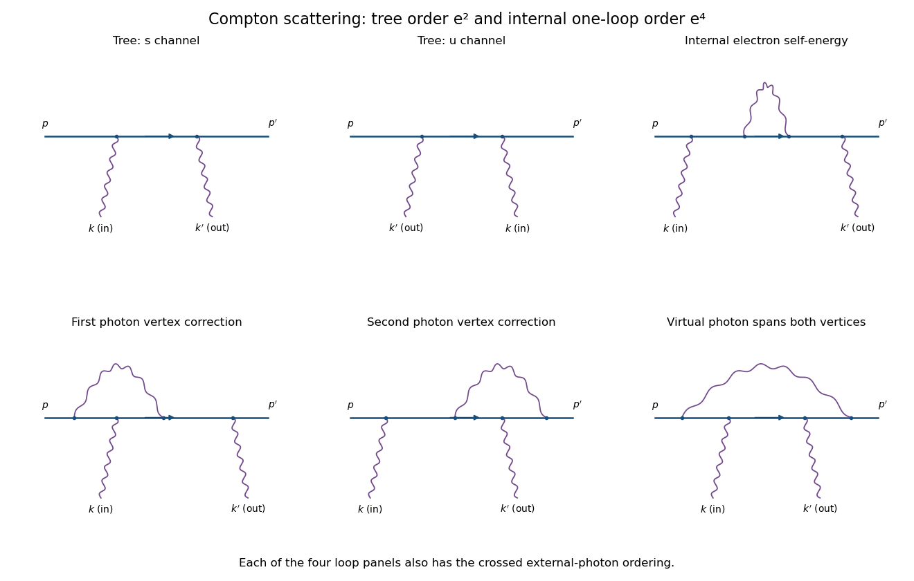
Compton tree diagrams and the four one-loop classes before exchanging the external photons
. Details. 
To prove the incoming Ward identity, replace by and write , with the Feynman boundary prescription understood. The physical nonzero-photon kinematics keeps these tree denominators off the electron pole. Sincethe external Dirac equations implyTherefore the two contracted terms are and its negative, and cancel. By linearity,This is the two-photon fermion Ward identity. An analogous cancellation holds for the outgoing photon. Gauge-equivalent polarization representatives have the same scattering amplitude, so a longitudinal pure-gauge component is not an extra physical photon state. Individual diagrams do not generally satisfy this identity; their sum does.
For perturbative order, each elementary QED vertex has one photon leg. If is the number of internal photon lines and , the vertex parity of a QED amplitude givesThus there is no third-order contribution. At fourth order, and, counting all three legs per vertex with four external legs, . A connected graph has loop number .
The nonzero one-loop classes on the open electron line are an internal-electron self-energy insertion, a vertex correction at either external-photon vertex, and a virtual photon spanning both photon vertices, giving the four-point box class. The first figure sketches each class for one photon ordering; interchange the two external photon attachments for its crossed partner. This yields two internal-self-energy graphs, four vertex graphs and two spanning-box graphs. They use the usual photon propagator, for example in Feynman gauge.
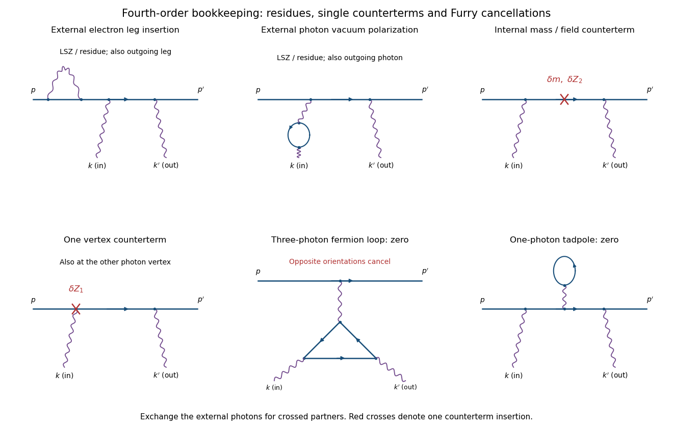
External-leg insertions, fourth-order counterterms and the odd-photon loops that cancel
. Details. 
For completeness, one-loop diagram classes for Compton scattering also depend on whether one is drawing an unamputated correlation function or a physical amplitude. Electron self-energies can be attached to either external electron leg, and photon vacuum polarization can be attached to either external photon leg, for both photon orders. In an on-shell renormalized S-matrix, these are accounted for by LSZ reduction and external-field residues rather than counted again as independent amputated graphs. Photon-leg corrections are not vacuum-polarization insertions on an internal Born photon: there is no such Born line.
At the same fourth order, a renormalized calculation has one mass or electron-field counterterm on the internal electron line, or one vertex counterterm at either Born vertex; the crossed partners are included. Each counterterm is a relative order- correction to the order- tree amplitude. External-field normalization must follow the same convention.
A possible closed electron loop with three photon vertices, linked to the external electron line by a virtual photon, cancels between its two orientations by Furry's theorem. Transposing the loop and using gives an extra sign , so its orientation-reversed partner is its negative. A one-photon tadpole likewise vanishes. Disconnected vacuum bubbles are removed by vacuum normalization. The first genuine radiative corrections are fourth order, with the internal self-energy, vertex and spanning-box classes and their consistently included renormalization terms.
Past exam of the mathematics course of the University of Cambridge 2004 iii Paper 44 2 Solution Created 2026-10-03 Updated 2026-10-14
For define . A fixed-coordinate infinitesimal field variation satisfying gives the Noether currentIndeed, the first variation issubtract the divergence of and use the Euler-Lagrange field equations. The components of the Lorentz four-vector are simply the field labels in this formula. For a transformation moving the coordinates, use its induced fixed-coordinate variation; this includes translations and Lorentz transformations. The spatial integral of is conserved when the spatial current has vanishing boundary flux.
With signature , a gauge transformation is . The electromagnetic field tensoris unchanged, since mixed derivatives of commute. Thus is gauge invariant. Write , so and . ThenThe overall minus sign produces a positive electric kinetic term and a positive physical Hamiltonian. Reversing it reverses the sign of the physical energy and gives the wrong positive-energy theory; the issue is the indefinite spacetime metric, not negative magnetic energy.
For , direct differentiation gives . Sincethe canonical energy-momentum tensor gives the conserved energy currentIts time component isbecause . Thus Noether's conserved canonical energy is . In pure, source-free electromagnetism the field equation gives , andFor sufficiently decaying fields, or boundary conditions removing this surface term,The canonical density is not locally gauge invariant, even though the total energy with these conditions is.
Now use the gauge-compensated time translation in electromagnetism,The extra term is a gauge transformation with the field-dependent parameter . It changes no field strength; therefore the combined variation still has and the same . The new current isIt is expressed entirely in gauge-invariant field strengths. In particularThis is the energy column of the electromagnetic stress-energy tensorin the chosen mostly-minus convention. Its conservation is the energy continuity equation.
The currents differ byon the source-free field equations. The final expression is an antisymmetric superpotential divergence, so it changes the integrated charge only by a boundary term. The compensating gauge transformation improves the local energy density without changing the physical conserved energy under the stated boundary conditions.
Past exam of the mathematics course of the University of Cambridge 2004 iii Paper 44 1 Solution Created 2026-10-03 Updated 2026-10-14
Use natural units and the Minkowski metric . The Lorentz group isWrite a transformation near the identity as . The defining relation gives , so is antisymmetric. ChooseThere are independent real parameters: three spatial rotations and three Lorentz boosts. Differentiating with respect to shows it is constant and equals . Thus exponentiating these infinitesimal generators gives Lorentz transformations connected to the identity. The component they generate is the proper orthochronous Lorentz group , characterized by and .
The local exponential calculation alone establishes products of exponentials. The single-exponential assertion also holds here. Use the Lorentz spinor double cover , obtained by acting on as . Its determinant is the Minkowski norm. A lift with distinct eigenvalues is diagonalizable and has a traceless logarithm with eigenvalues , where . With repeated eigenvalues, choose between and so that the lift is with ; its traceless logarithm is . Since the two signs have the same Lorentz image, exponentiating the differential of the covering map proves every proper orthochronous Lorentz transformation is an exponential:It is not a global assertion about the disconnected improper components of .
For Dirac spinors, choose gamma matrices satisfying the Clifford algebra and setThe Clifford relations giveThey also give the stipulated Lorentz commutator with every replaced by : commute through the two gamma factors defining the other generator and collect the four terms. Consequently this is a representation of the Lie algebra of the Lorentz group, and exponentiation yieldsThe Dirac adjoint transforms as , since .
There is a global qualification: a spatial rotation through gives , while its Lorentz matrix is . Thus Dirac spinors form an ordinary representation of the double cover, and a double-valued representation of , rather than a single-valued linear representation of itself. Fermion bilinears are unaffected by this sign.
For a scalar field, and its derivative transforms as a covector. A Lagrangian density must have all Lorentz indices contracted into scalars using invariant tensors; arbitrary scalar potentials are allowed. For example the kinetic contraction and a potential are invariant. Lorentz invariance by itself does not restrict the potential to quartic order: that restriction would be an additional four-dimensional power-counting requirement.
Define . It commutes with all , so the axial current transforms as a vector under . Hence all three proposed contractions are invariant under . If invariance under parity or the full improper Lorentz group is also required, the distinction is:The axial current is a pseudovector: under an improper Lorentz transformation it has the extra determinant sign. The mixed derivative–axial contraction is therefore a pseudoscalar, while the square of the axial current has two cancelling signs. If is itself a pseudoscalar, its derivative supplies the second sign and the mixed coupling becomes parity even. This is the axial derivative coupling and parity distinction; parity invariance must not be silently assumed from proper Lorentz invariance.
In four dimensions, , and . The three operators have mass dimensions , respectively. Thus the latter two require dimensionful couplings and are not power-counting renormalizable interactions, but this does not invalidate their Lorentz invariance or their use in an effective field theory.
Past exam of the mathematics course of the University of Cambridge 2004 iii Paper 43 4 Solution Created 2026-10-03 Updated 2026-10-14
princomp(): principal component analysis. Supply observations in rows and numeric variables in columns. After centering, let denote the resulting matrix and its sample covariance matrix, with an explicitly stated normalization. WriteThe first direction maximizes the Rayleigh quotient over unit vectors; successive directions maximize it subject to orthogonality to the earlier directions. The principal component scores are , with variances and zero pairwise sample covariance. Zero covariance alone does not imply independence. Each principal component loading describes a direction in variable space; its sign is arbitrary, and repeated eigenvalues leave the basis inside the corresponding eigenspace arbitrary.The function returns principal component loadings, component standard deviations
sdev and, when requested, principal component scores. By default it uses a covariance matrix; cor=T instead performs principal component analysis on a correlation matrix, standardizing nonconstant variables to variance one. This choice matters when variables have different measurement units. These interface details are documented in the S-Plus help for princomp.A scree plot shows the ordered eigenvalues; a plot of the first two principal component scores can reveal groups, unusual observations or a dominant gradient. The first components explain of the total variance. Reconstructing each centered observation by its orthogonal projection onto these directions minimizes average squared reconstruction error among -dimensional linear subspaces. Thus PCA gives an optimal linear compression for squared reconstruction error, with scaling and the retained dimension chosen explicitly. It is an unsupervised learning method, rather than a classification rule fitted to supplied labels.
tree(): classification trees and regression trees. A call such as tree(response ~ predictors, data=dat) fits a recursive partitioning model. At a current node, test numerical predictors against candidate thresholds, or divide the levels of a categorical predictor into two sets. Select a split that most improves the fitting criterion, then repeat within its children. Numerical splits give axis-aligned regions. A categorical response produces a classification tree; a numeric response produces a regression tree, as specified in the S-Plus tree documentation.For a regression tree, the constant prediction in a terminal region is its sample mean, minimizing the sum of squared residuals there. For a classification tree, estimate class probabilities by the observed proportions in a leaf and predict a most probable class under equal misclassification costs. The classification-tree deviance of a node iswith ; splitting maximizes the decrease from parent to children. This fitting criterion differs from the number of wrong classifications. The middle sketches show the same three-region partition as a binary tree: first split on variable one, then split the right-hand branch on variable two.
Growing to small leaves can overfit. Use cost-complexity tree pruning, balancing fitted loss against leaf count,and select complexity by cross-validation. Plotting the fitted tree and annotating nodes displays the rules; prediction routes each new observation through the fitted splits. A tree gives an interpretable, piecewise-constant prediction rule; training fit alone does not measure prediction accuracy.
The
rpart() alternative. This also fits classification and regression trees by recursive partitioning, with squared-error splitting for ordinary numeric responses and, by default for classification, Gini impurity . Classification settings can instead use information-based splitting and specify prior probabilities and a loss matrix. It supports surrogate splits to approximate a node's primary left/right assignment when the primary predictor is missing. Its complexity-parameter path and cross-validated errors support cost-complexity tree pruning; for example, select a complexity parameter and apply prune(fit, cp=...). The maintainer's rpart documentation describes the criteria and the distinction in handling surrogate predictors. The partition and tree sketches apply to either implementation; the fitted tree need not be the same because splitting criteria and controls can differ.cmdscale(): classical multidimensional scaling. Its input is a dissimilarity matrix or stored distance object. It outputs coordinates for the observations in a chosen dimension, usually two for visualization. Let contain the squared entries of , and putFor centered Euclidean coordinates , the distance identity gives : multiplying by removes the row and column norm terms. Diagonalize this Gram matrix and retain its largest positive eigenvalues. The coordinates areThus classical scaling exactly recovers Euclidean distances when all positive eigenvalues are retained. Reducing dimension approximates the centered Gram matrix; it does not in general minimize squared discrepancies in the original distances. Negative eigenvalues identify a failure of the Euclidean distance matrix criterion, so their size matters when interpreting a display. The historical S-Plus cmdscale help describes the dimension argument, eigenvalue output and optional additive adjustment to dissimilarities.Plot the two coordinate columns on equally scaled axes and label observations. Nearby plotted points suggest small dissimilarities only insofar as the dimension reduction fits the input well. The bottom sketches give an exact Euclidean example: a configuration and its independently recovered two-dimensional coordinates have identical pairwise distances, despite different coordinate axes. Classical scaling converts distances into geometry; translations, rotations and reflections do not change the represented distances. For Euclidean distances between observations, its coordinates agree with the corresponding principal component scores up to these harmless choices of axes.
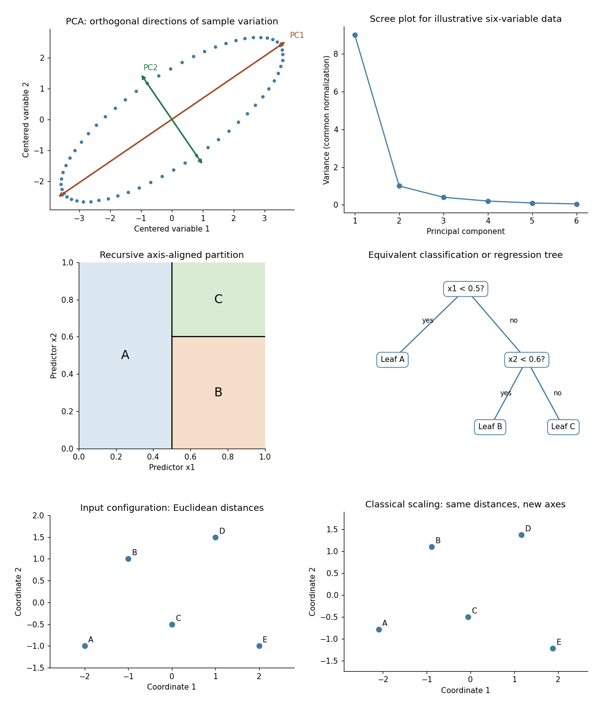
Illustrative PCA directions and scree plot, equivalent recursive partition and tree, and exact classical-scaling recovery of Euclidean distances
. Details. 
There are unlisted articles, also show them or only show them.