
Past exam of the mathematics course of the University of Cambridge 2004 iii Paper 43 3 Solution Created 2026-10-03 Updated 2026-10-14
The first command reads a rectangular data file into
a; header=T treats the first line as variable names. There are twelve observations, identified by student names, and nine binary attributes. A one records presence of an attribute and a zero records absence. This is a description of the encoding, not a claim that every presence is equally important for a scientific application.dist(a, metric="binary") compares rows using Jaccard distance. If counts shared presences and count mismatched presences, thenJoint absences do not enter the denominator, unlike the simple matching coefficient or normalized Hamming distance. dist2full(d) expands the stored pairwise distances into a symmetric dissimilarity matrix; round(...,2) changes only its displayed precision. The clustering command still receives the original unrounded distances.For example, Tom and Martin have six shared presences and only one mismatch, giving . Taeko and Luitgard have three shared presences and four mismatches, giving . LingChen and Mohammad share only the meat attribute and differ on four others, giving . The diagonal is zero, and the entries are symmetric because exchanging the two observations exchanges and .
hclust(d, method="compact") constructs an agglomerative hierarchical clustering object by complete-linkage clustering. Its distance between two current groups isStart with singleton groups, merge a pair with smallest intergroup distance, update these maximum cross-pair distances, and repeat until one group remains. The object stores the merge structure, merge heights and a leaf order suitable for a dendrogram; assigning it to h does not itself display a graph. The historical S-Plus help identifies compact with complete linkage and describes the plotting object.The first merge is Tom with Martin at . At the next height , either LinYee with HuiChin or HuiChin with Meg may merge: the distances are tied. The following dendrogram shows one valid resolution, using original row order to resolve ties. In this tree, LinYee joins HuiChin at , Pio joins Meg at , and Nicolas joins Tom–Martin at . The latter height is , illustrating the complete-linkage update.
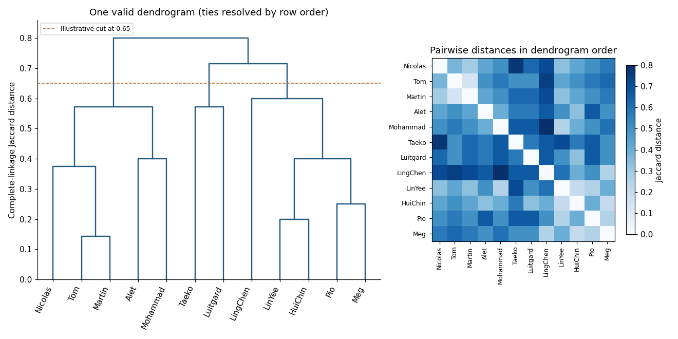
Complete-linkage dendrogram and Jaccard-distance heatmap for the binary student profiles, with one valid tie convention
. Details. For the displayed tree, a cut at height gives three groups: Taeko–Luitgard; Alet–Tom–Martin–Nicolas–Mohammad; and LinYee–Pio–LingChen–HuiChin–Meg. The last two merges occur at and . The hierarchy is a description under the chosen binary distance and linkage rule; it neither supplies an intrinsically correct number of groups nor guarantees a unique tree in the presence of ties. Changing the treatment of joint absences, or the weighting of attributes, can change that description.
Past exam of the mathematics course of the University of Cambridge 2004 iii Paper 42 6 Solution Created 2026-10-03 Updated 2026-10-14
In a regular model let be the log-likelihood, its score, its total Fisher information, and the unrestricted maximum-likelihood estimator. For a point null in a p-dimensional parameter space, the standard statistics areThese define the Wald test, score test and likelihood-ratio test. With an interior true parameter, increasing information, suitable differentiability and asymptotic normality, all have asymptotic chi-squared distribution with p degrees of freedom under the null. Observed information can replace expected information when it is asymptotically equivalent.
For q smooth independent restrictions , replace the Wald statistic by , where G is the derivative of g at the estimate; compare with chi-squared q. The likelihood-ratio statistic uses the difference between unrestricted and null-restricted maxima. The score statistic is computed at the restricted maximum and uses efficient information for the tested coordinates: with nuisance coordinates lambda this is . Inverting the acceptance inequalities for point nulls produces approximate coverage- confidence regions; for example the Wald region consists of theta satisfying . Analogous score and likelihood-ratio inequalities give their confidence regions.
For the Poisson family, put to include the initial observation, and defineMultiplying the initial and conditional Poisson probabilities gives, on the supported observation sequences,The parameter-free term is , interpreting as zero. A positive count after a zero preceding count is outside the support.
For , strict concavity gives unconstrained maximum , and the upper endpoint restriction givesThere is an endpoint qualification in the printed question. With probability , and all later counts are zero. Then , and the likelihood is , which has no maximum on the stated space . The formula produces zero only as an extended estimate on the closure . This is a likelihood supremum at an excluded boundary, and zero cannot be called an actual maximum in the original space.
The observed negative second derivative is . Conditional expectation gives and . Therefore for ,This is the bounded information in a subcritical Poisson branching process. Observing more generations of one family does not provide unbounded information. Indeed , and zero is absorbing, so extinction occurs at a finite generation almost surely. The total observed progeny is finite; eventually , , and the extended estimate equals , a discrete nondegenerate random variable rather than a consistent increasingly precise estimate.
Here is a direct proof of the failure of a chi-squared Wald limit which does not rely solely on the information bound. Under any interior null , the event , has probability and forces every later count to be zero. On it the genuine constrained estimate is for every , so the usual expected-information Wald statistic isThus it has a persistent atom tending to . The fact that atoms obstruct a continuous distributional limit rules out a chi-squared limit, including when equals one half and that atom is at zero. Any definition adopted for the separate all-zero sample event leaves this positive-count counterexample intact. Hence the Wald statistic does not have the usual asymptotic chi-squared null law for this increasing observation horizon.
Past exam of the mathematics course of the University of Cambridge 2004 iii Paper 42 5 Solution Created 2026-10-03 Updated 2026-10-14
A marginal statistical likelihood uses a statistic whose marginal sampling distribution depends on the parameter of interest but does not involve the nuisance parameter. It integrates out other observed coordinates. A profile likelihood instead keeps the full data and, for every fixed interest parameter, fits the nuisance parameter by maximizing the full likelihood. Profiling supplies a likelihood function but usually not a normalized sampling probability density function. Here the marginalization is of data coordinates; Bayesian model evidence averages parameters against a prior and is a separate construction.
Use shape-rate notation for the gamma distribution. The independent sums have and , so their joint probability density for isFor , the absolute Jacobian determinant is u. ThereforeIntegrate u using the gamma integral . The lambda factors cancel, leavingThus T gives a nuisance-free marginal likelihood. Discarding only terms independent of psi, its logarithm isThe factor t in the logarithm is required, as in the original PDF.
The full log-likelihood is . Its lambda derivative vanishes uniquely atThe second derivative in lambda is negative. Substituting this maximum gives . Since , it agrees with up to a psi-independent constant. This proves the Gamma-ratio marginal and profile likelihood identity. Their common maximizer is , if an interest-parameter estimate is also wanted.
Past exam of the mathematics course of the University of Cambridge 2004 iii Paper 42 4 Solution Created 2026-10-03 Updated 2026-10-14
Assume a symmetric second-order probability density function kernel for density estimation and enough smoothness for the displayed derivative functionals. The benchmark smoothing bandwidth is , balancing against . Three widely used selection methods are as follows.
For least-squares density cross-validation, expand integrated squared error as . Estimate the middle integral by leaving out the observation at which the estimate is evaluated, and minimizeThe left-out observation is independent of its estimator, so the second term has expectation . Thus exactly. The subtraction of the self-contribution is essential. Computation uses , where . This method directly targets integrated error without estimating a curvature functional first. Under standard smoothness and a suitable search interval its selected smoothing bandwidth is ratio-consistent with the MISE optimum, and hence with . Relative fluctuations are ordinarily , so the selected values can be quite variable in finite samples.
For biased density cross-validation, estimate curvature from the second-derivative probability density function estimator and subtract its diagonal variance term:Differentiating the kernel for density estimation estimator and applying the integrated-variance identity gives the exact expectation . Under the derivative regularity assumptions, , so . Minimize BCV over a reasonable smoothing bandwidth range. It is a smoothed criterion directed at AMISE; the name reflects its finite-sample bias rather than an exact unbiased-risk identity. Standard conditions again give ratio consistency and relative fluctuation order . It often has a smoother objective than ordinary least-squares cross-validation, though numerical behavior and relative variance depend on the probability density function and kernel for density estimation.
For plug-in bandwidth selection, obtain an independent pilot scale g, estimate , then setThe pilot should be positive and stable; consistent positive estimates make this expression ratio-consistent by continuity. A simple normal-reference initialization uses under a normal reference model, substituting a sample scale for sigma. For a Gaussian density kernel this gives . A pure normal-reference rule is quick but is asymptotically correctly calibrated only when its assumed curvature matches the actual probability density function; it is useful as the first stage of a data-driven plug-in procedure.
A more adaptive fourth-derivative pilot estimate of density curvature uses , obtained by two integrations by parts, and estimates it byThe diagonal expectation contributes ; the leading smoothing bias is . Balancing these terms produces the stated pilot scale , with another pilot or reference model supplying . Under sufficient derivatives and tail control, its error is bounded byat that pilot scale. Taylor expansion of the fifth-root formula gives , so it inherits that bound. A calibrated cancellation of leading pilot bias can give a faster rate. This illustrates why an appropriately constructed plug-in selector can converge more quickly than cross-validation, while requiring more smoothness and pilot choices. For each ratio-consistent method, its attained AMISE divided by the minimal AMISE tends to one.
Past exam of the mathematics course of the University of Cambridge 2004 iii Paper 42 3 Solution Created 2026-10-03 Updated 2026-10-14
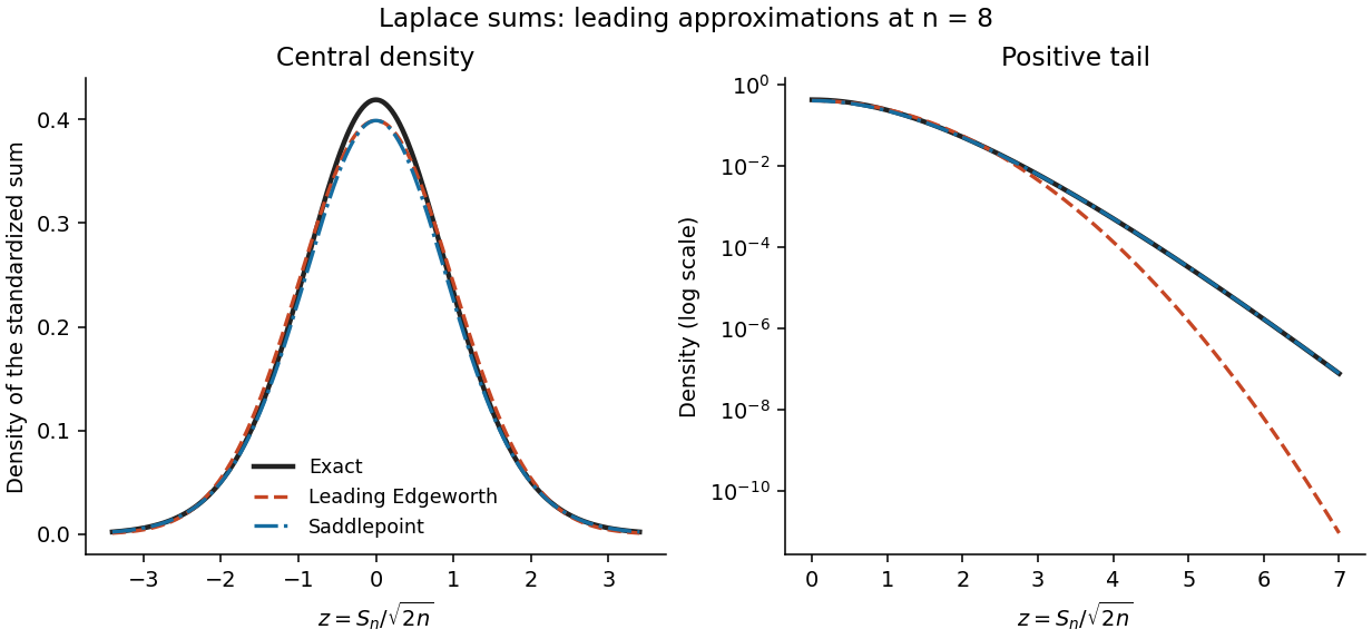
Let the summands have mean mu, variance , and cumulants . For the standardized sum , expansion of its log-characteristic function gives a normal leading term and successively smaller cumulant terms. Fourier inversion turns these terms into Probabilists' Hermite polynomials. Under sufficient moments and a smooth nonlattice condition, the Edgeworth expansion beginsfor bounded z. Higher orders include the fourth cumulant and products of lower cumulants. This is a central expansion in powers of ; it need not remain positive, normalized, or accurate in far tails after truncation.
For a saddlepoint density approximation, require the summand cumulant-generating function K to be finite on an interval about zero. At a sum value , find the interior saddle satisfying . Exponential tilting makes the tilted mean y, so the tilted sum is approximated locally by its normal probability density at its mean. Undoing the tilt givesEquivalently this follows by deforming the transform-inversion contour through its stationary point. Suitable analytic and nonlattice regularity gives relative error at fixed interior y. This approximation incorporates a nonquadratic tail exponent and is positive, while an Edgeworth truncation uses a normal probability density times a polynomial. It uses more information from the distribution and stronger exponential-moment assumptions. Its integral may differ from one by a higher-order amount, so positivity does not imply exact normalization.
For the centered Laplace distribution, , hence and . Its skewness vanishes, so the order- Edgeworth correction is zero. With , the requested expansion, omitting terms of order in the standardized correction, isFor bounded z the exact probability density function is this expression times . The prefactor is because this is the probability density function of the unstandardized sum; that change of units should not be confused with the orders inside the Edgeworth expansion.
For the saddlepoint, . Write and . The root in isThese formulas include without a division by y. Substitution yieldsThis is the leading saddlepoint approximation, without its order- relative correction. Expanding d near one recovers the same central normal approximation, while retaining d captures the Laplace-sum large-deviation exponent away from the center.


Past exam of the mathematics course of the University of Cambridge 2004 iii Paper 42 2 Solution Created 2026-10-03 Updated 2026-10-14
The empirical distribution function is . For continuous F, the probability integral transform gives independent uniform variables . Strict increase of F is unnecessary. More explicitly, generate the observations by with the generalized quantile inverse. Then , so , where is the uniform empirical distribution.
Continuity and the limits of F ensure that its range contains . The endpoint discrepancies for are zero. Hencewhich depends only on n. Equivalently it is , a function of uniform order statistics. This proves the distribution-free property of the Kolmogorov-Smirnov statistic even when F has flat portions.
Choose from this common distribution so that . The Kolmogorov-Smirnov confidence band isThe event that all these inequalities hold is exactly the event used to choose the critical value, giving simultaneous coverage . The Glivenko-Cantelli theorem states that for an independent identically distributed sample from any distribution function, continuous or not, almost surely.
For an integrable r-argument U-statistic kernel, replace it by . Every permutation has the same expectation by exchangeability, so this symmetrization of a U-statistic kernel preserves the target functional. For a symmetric U-statistic kernel h and , the U-statistic isEach summand has expectation theta, hence the statistic is unbiased.
For the population variance, use . Independence gives when the second moment is finite. The corresponding statistic simplifies using :Thus variance as a U-statistic is precisely the usual unbiased sample variance, for .
Past exam of the mathematics course of the University of Cambridge 2004 iii Paper 42 1 Solution Created 2026-10-03 Updated 2026-10-14
A kernel for density estimation is an integrable function K of unit integral, ordinarily nonnegative and centered. Square integrability is needed for integrated variance; a symmetric second-order kernel for density estimation also has and finite nonzero second moment . Its scaled form is , and the kernel density estimator isHigher-order signed kernels are possible, but need not give a nonnegative probability density function estimate.
The mean integrated squared error is . Put . Independence gives the pointwise mean and variance . Integrating, use and Fubini to obtain . The bias-variance decomposition proves the exact formulaEquivalently this is . These identities assume the displayed integrals are finite; they are exact, rather than a small-smoothing bandwidth expansion.
For a symmetric second-order kernel for density estimation, Taylor expansion gives leading bias , and the leading integrated variance is . Thus the asymptotic mean integrated squared error balances inverse smoothing bandwidth against fourth-power bias, with optimal smoothing bandwidth . Its appearance of the integrated squared density curvature motivates the scale comparison.
For , , two differentiations give . A change of variables therefore gives , which tends to zero as if the original curvature integral is finite. The distribution with probability density function is that of X divided by a, so . ConsequentlyThis scale-invariant density curvature measures shape without dependence on the units used to measure X.
For the final minimization, write and use the triweight kernel on , zero outside. Integration gives total mass one, mean zero and variance . Its value and its first two derivatives vanish at both endpoints, so its extension is twice continuously differentiable. On the interior,In particular and .
Put . The mass and moment constraints give , since both means vanish and their variances match. If the claim is immediate; otherwise expand the squared norm and integrate its cross term twice by parts over . The first endpoint term vanishes because , but the next one must be retained:For the second equality use the zero mass and second moment of e and outside the support. All terms in the last expression are nonnegative, including the endpoint values of a probability density function. It follows thatThis proves that the triweight density minimizes integrated squared curvature under the specified constraints. Equality forces ; a globally affine integrable difference of probability density functions is zero, so equality occurs only at .
Past exam of the mathematics course of the University of Cambridge 2004 iii Paper 41 4 Solution Created 2026-10-03 Updated 2026-10-14
Use the shape-rate convention for the gamma distribution , with prior distribution probability density function proportional to . The observations are independent conditional on the common parameter . Unconditionally a common nondegenerate prior distribution induces covariance between distinct observations, so the Bayesian inference model requires conditional independence.
For unit-exposure counts, the likelihood is proportional to . Multiplying by the prior distribution givesThe future count has conditional expectation , so posterior distribution averaging givesThis is an exact Bayesian credibility estimate, with credibility factor and collective mean .
For the insurance exposure and claims inflation calculation put , assuming , and positive policy counts . Let be the total claim count in year . Conditional independence of the policy counts gives , and the observed average amount satisfiesFor possible observations, the recovered are nonnegative integers. If they are not, the data have zero likelihood under the model and no conditional posterior distribution is defined for those impossible values.
Write and . Since and determine each other, conditioning on the observed average amounts is equivalent to conditioning on these counts. The independent yearly count likelihood isThe Poisson-gamma conjugacy with unequal exposures therefore givesFor the future year, ; the number of future policies cancels because is a per-policy average. HencewithThe collective mean is the prior distribution expected claim amount per policy in the future year's monetary units. The experience mean first inflates each past per-policy amount to that same future year and then averages with policy-exposure weights. Equivalently, it estimates annual claim frequency by total observed claims divided by total past insurance exposure and converts that frequency to the future claim cost. This is inflation-adjusted Poisson-gamma credibility.
For fixed prior distribution parameters, increases strictly with total past insurance exposure: , and as . The prior distribution weight decreases to zero; acts as equivalent prior distribution insurance exposure. With no past insurance exposure the appropriate weight is zero and the prediction is , without defining an empirical experience mean.
Past exam of the mathematics course of the University of Cambridge 2004 iii Paper 41 3 Solution Created 2026-10-03 Updated 2026-10-14
For nontrivial positive claim sizes in the classical risk model and , the adjustment coefficient is the unique positive solutionIndeed, has , , and is strictly convex. It becomes positive near the right endpoint of the moment-generating function domain. For a finite endpoint this follows from the assumed divergence; for an infinite endpoint, for some gives an exponential lower bound on , which eventually exceeds any linear function. Convexity gives existence and uniqueness of the positive crossing and .
Put and . Substituting into the supplied survival renewal equation for a classical risk model, and using , yieldsMultiplying by gives the proper renewal-type equationThe exponential tilt of the ruin renewal kernel turns a defective kernel into a probability density function, because the tail integration identity givesThis identity follows also by integrating and applying Tonelli theorem. The tilted probability density function defines a nonarithmetic distribution, even if the claim size probability distribution itself has atoms.
Differentiate to calculate its mean:It is finite and positive because is inside the finite moment-generating function domain. Next, reversing the order of integration givesThe forcing function is directly Riemann integrable. Choose with . Markov's inequality bounds by , so is bounded by a constant times . It is continuous; on finite intervals continuity controls its Riemann sums, and the exponential envelope controls the tails. These are sufficient conditions for direct Riemann integrability.
Iterating the renewal equation by convolution gives , where is the renewal measure. The remainder after iterations is bounded on each fixed interval by a constant times the chance that a sum of positive interarrivals remains in that interval, which tends to zero. The key renewal theorem, applicable to this nonarithmetic distribution of finite mean and the directly integrable forcing, now gives the interior adjustment coefficient ruin prefactor:Both numerator and denominator are positive, so .
For the unit-rate shape-two Erlang distribution, , and . Write , so positive loading requires . Dividing the adjustment coefficient equation by its nonzero root gives . ThusThe last simplification uses ; it is the Erlang shape-two ruin prefactor. Its value depends on the premium-to-arrival ratio, which is not specified numerically.
For the final exponential representation, evaluating at zero in the survival renewal equation for a classical risk model gives . If the slower term is present, necessarily and . Comparing with the finite positive asymptotic constant just proved yieldsA smaller adjustment coefficient would make the limit zero and a larger one would make it infinite. Here the leading exponential term determines a ruin adjustment coefficient. The coefficient need not be assumed positive to identify the leading term.
The wording does not specify that is nonzero. If and , the only surviving term instead gives , and . This case is realizable: claims with an exponential distribution of rate have ultimate ruin probability . Negative would make the ultimate ruin probability negative for large , and both coefficients zero are incompatible with a nontrivial positive claim rate and mean. These observations specify the coefficient qualification needed for the usual answer.
Past exam of the mathematics course of the University of Cambridge 2004 iii Paper 41 2 Solution Created 2026-10-03 Updated 2026-10-14
Let . Conditioning on givesWhere the moment-generating function is finite around zero, differentiating the cumulant-generating function givesIn particular and . These compound Poisson cumulants use raw claim moments. The first two formulas also follow by conditioning: and , soThis is the law of total variance. They therefore remain valid with finite first two moments even when no positive exponential moment exists.
Under per-claim excess of loss reinsurance, put and let be the positive part of the excess. The insurer and reinsurer totals are sums of these payments over the same Poisson distribution count. Write . Using the tail integral formula for moments on the tail probabilities of and givesFor example, after , and shifting by gives the reinsurer formula. The moment formulas are finite whenever the corresponding claim moments are finite.
For the specified Pareto distribution, with shape three and minimum ,If , every claim exceeds the reinsurance retention. ThereforeIf , the tail integrals instead giveConsequently the requested sum of variances isOn the first branch, ; it decreases until and then increases. On the second branch . For the minimum is unique; if , all variances are zero and every reinsurance retention minimizes them. ThusThe curve starts at , reaches this minimum, passes through with matching slope on both branches, and then increases concavely toward the horizontal asymptote . The variance-minimizing retention for shape-three Pareto claims is shown below.
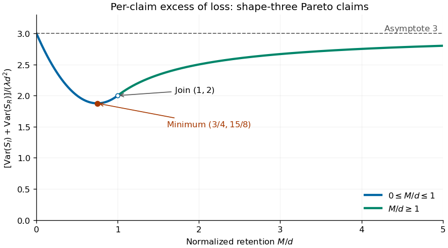
Sum of insurer and reinsurer aggregate variances for shape-three Pareto claims, minimized at retention three quarters of the minimum claim size
. Details. 
The two aggregate payouts are dependent. Conditioning on the common count gives covariance , so for every reinsurance retention, as required by . The covariance of two components of a compound Poisson sum accounts for this distinction between a sum of variances and the variance of a sum.
There is a moment domain qualification for this heavy-tailed example. For every , , and moments of order also diverge. Thus its positive moment-generating function is not finite and higher finite cumulants cannot be obtained by differentiating around zero. Its mean and variance calculations above are valid by conditioning or by the first two right derivatives at zero of the Laplace transform of a nonnegative random variable.
There are unlisted articles, also show them or only show them.