For sequences indexed by the integers, discrete convolution adds products whose indices sum to the output index:For finite sequences, treat every unspecified entry as zero; the sum then has finitely many nonzero terms. For infinite sequences, a convergence hypothesis is needed, for example absolute summability of both sequences.
Take at indices and at indices . Their convolution is at indices :Equivalently, : add an unshifted and a one-step shifted copy of . This explains the output by superposition, with every index included.
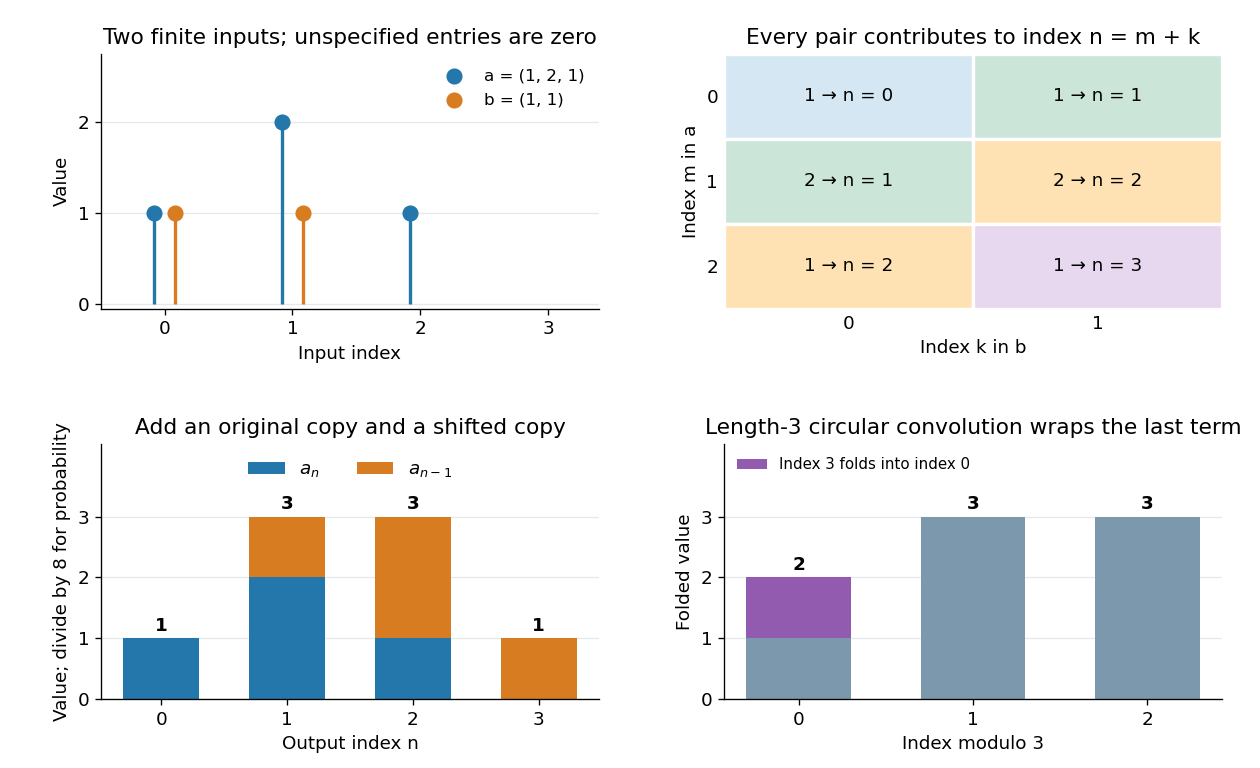
Discrete convolution combines index pairs, shifted copies, polynomial coefficients and outcome counts
. Details. 
The same products appear in polynomial multiplication and generating functions:A term times contributes to coefficient , precisely the index condition in discrete convolution. In probability, counts the outcomes of two independent fair coin tosses by their number of heads, while counts the outcomes of one more toss. Dividing the output by eight gives the probability mass function of the binomial distribution with and . No new arithmetic is needed to pass from coefficient multiplication to counting independent sums.
The full finite convolution is different from circular convolution, where indices wrap modulo a chosen length. Wrapping this four-term output to length three adds its last entry to its first and gives . When using a discrete Fourier transform to compute the full convolution, zero padding to length at least the sum of the input lengths minus one prevents this wraparound. [ref]
https://ocw.mit.edu/courses/res-6-008-digital-signal-processing-spring-2011/610905d8154ec2bfc090cf78022249a5_MITRES_6_008S11_lec10.pdf. Oppenheim, MIT Digital Signal Processing, Lecture 10, circular convolution and zero padding
A standard approximate identity on is a family withThe absolute tail condition matters for signed or complex kernels: cancellation of the signed mass alone is insufficient. For and , these conditions imply .
Indeed, express the difference as . Translation continuity in Lp makes the integrand norm small near zero, the uniform L1 norm controls that part, and the vanishing absolute tail controls the remainder. The same proof gives uniform convergence for bounded uniformly continuous functions. It does not give norm convergence for every essentially bounded function.
For nonnegative normalized mollifiers with smooth compactly supported , convergence also holds at every Lebesgue point of a locally integrable function. Such pointwise conclusions use additional size control on the kernels; they should not be attributed to the three norm-approximation conditions alone. The Cauchy approximate identity and summability kernel on the circle are related constructions on their respective domains.
For a function , its perspective isIf is convex, so is jointly in . For two domain points and , put and . ThenApply convexity of and multiply by to obtain the required convexity inequality for . The weights are rescaled by the positive , not left equal to and .
Convexity domain of x cubed plus y cubed plus Axy by  Codex 0 Created 2026-09-24 Updated 2026-10-05
The Hessian matrix ofis positive semidefinite exactly whenThis region is convex: for it is the epigraph of in the positive quadrant, and for it is the closed first quadrant.
A finite convex function on an open convex subset of a finite-dimensional real vector space is locally Lipschitz, and therefore continuous. In one dimension this follows by bounding its secant slopes between two slightly wider endpoints.
If a convex subset of is invariant under cyclic coordinate permutation, averaging the cyclic images of shows thatalso belongs to the set.
Let have the binomial distribution with trial count and success Probability . If , thenThis is the Poisson limit theorem: many independent rare trials retain a finite total expected count. For a proof using characteristic functions,The logarithmic expansion error vanishes because . The limit is the Poisson distribution characteristic function, so the Lévy continuity theorem proves convergence. The case is the degenerate count zero; it also follows directly from Markov's inequality.[ref]
Probability: Theory and Examples (fifth edition) by Rick Durrett. Section 3.6, Theorem 3.6.1 and its characteristic-function proof
For example, is approximated by , and its zero-count Probability is about , close to . The limiting mean is the limit of the product, not either individual parameter. independent unequal-probability Bernoulli trials have a related Poisson approximation when their largest success Probability vanishes and their total mean converges; dependence requires additional control, as in the Stein-Chen method.
Let be real independent and identically distributed random variables with expected value and finite, strictly positive variance . Write and for their sum and sample mean. The central limit theorem statesPrecisely, for every real ,where is the standard normal distribution function. The conclusion is convergence in distribution to the standard normal distribution. If the variance is zero, every observation equals almost surely; the displayed normalization is then undefined and there is no fluctuating error to describe.
The striking feature is that the observations need not have a normal distribution. They may be binary, bounded, or strongly skewed. Their detailed probability distribution disappears from this limit except through the expected value and variance. The subtraction removes predictable growth: . The division implements variance normalization: variance additivity for independent random variables gives , so every has expected value zero and variance one. For nonzero , an uncentered sum drifts; without rescaling its spread grows.
For a concrete example, let each have a Bernoulli distribution with success probability . Then has a binomial distribution, with expected value and variance . Its exact probability mass function and its normalized count areHere is a binomial coefficient. Individual trials are conspicuously skewed, yet their centered, rescaled counts approach the same standard normal distribution as sums of fair trials.
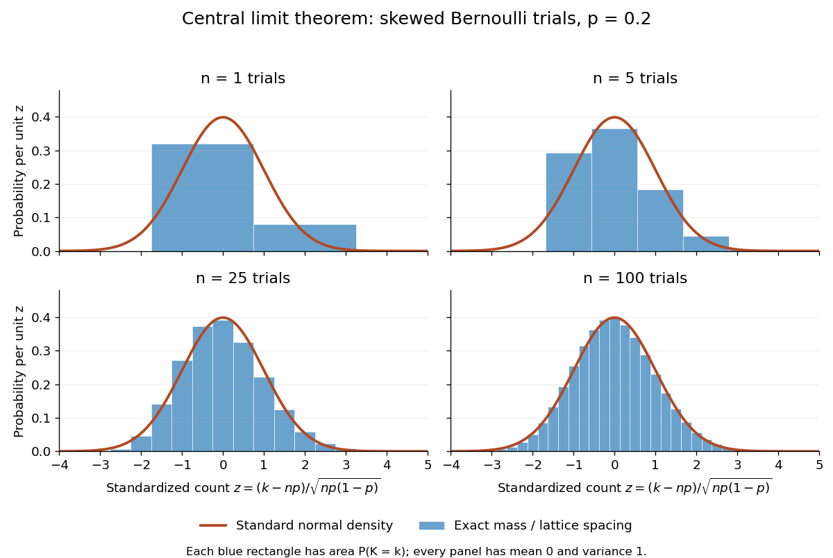
Exact standardized binomial distributions approach the standard normal curve
. For independent Bernoulli trials with , each blue bar has width equal to the normalized lattice spacing and area equal to the exact binomial distribution mass at its center. Heights are mass divided by spacing, so they can be compared with the orange probability density function of the standard normal distribution. All four normalized counts have expected value zero and variance one. The rectangles visualize discrete masses; they do not make the discrete probability distributions continuous. Details.
At , has expected value and standard deviation . The exact binomial distribution gives . A normal approximation with the continuity correction uses the interval to :The small discrepancy is an approximation error, not an equality supplied by the central limit theorem.
The strong law of large numbers and weak law of large numbers locate the average: , respectively by almost sure convergence and convergence in probability. The central limit theorem magnifies that shrinking error and describes its shape. In terms of the sample mean, the resulting normal approximation is , with standard error . This explains why four times as many independent observations halve the standard error. When is known, has approximately coverage for at large , giving a confidence interval. This coverage refers to repeated samples, not a guarantee for an individual interval.
A useful application is the Monte Carlo method: estimate a success probability by the proportion of successful simulated trials. Nicholas Metropolis and S. Ulam's original paper, "The Monte Carlo Method" (1949), illustrates this with games of solitaire and estimation of a region's volume by randomly selected points, and discusses why estimates require probabilistic error control. The strong law of large numbers justifies convergence of such proportions for independent repetitions; the central limit theorem supplies their large-sample error scale when .[ref]
https://hedibert.org/wp-content/uploads/2013/12/1949MetropolisUlam.pdf. Metropolis and Ulam, The Monte Carlo Method, JASA 44 (1949), 335–341, especially pp. 336–337
There are three useful limits to this picture:
- A heavy-tailed distribution can have infinite variance, so the displayed hypothesis must be checked. A Pareto distribution with minimum one and shape has finite expected value three but infinite variance. The strong law of large numbers still applies, but the stated central limit theorem does not. More dramatically, the Cauchy sample mean has an unchanged distribution: even averaging need not concentrate when the expected value is undefined. A heavy-tailed distribution with finite variance is allowed by the stated central limit theorem.
- Independence matters. If all equal the same nonconstant Bernoulli random variable, then and . There is no accumulation of new information, and the variance of the sum grows like , not . Other versions of the central limit theorem can allow dependence, but require hypotheses controlling it.
- Convergence in distribution is a limiting assertion, with no universal sample size or error rate under finite variance alone. It does not automatically give accurate relative estimates of very small tail probabilities. Nor does it mean that discrete point masses converge as probability density functions: a binomial distribution remains discrete for every finite . If the success probability changes with so that and , the relevant result is the Poisson limit theorem, rather than the fixed- argument above.
A historical original-paper reference is J. W. Lindeberg's "Eine neue Herleitung des Exponentialgesetzes in der Wahrscheinlichkeitsrechnung" (1922), published in Mathematische Zeitschrift 15, pp. 211–225. The Lindeberg condition and Lindeberg-Feller central limit theorem below describe a version for sums whose summands need not share a probability distribution.[ref]
https://doi.org/10.1007/BF01494395. Lindeberg, Eine neue Herleitung des Exponentialgesetzes in der Wahrscheinlichkeitsrechnung (1922)
A brief proof outline uses the characteristic function of . Its expected value is zero and its variance is one, so the finite second moment givesThe Taylor expansion of the complex exponential, with its remainder controlled by , and the dominated convergence theorem justify this step without a third-moment assumption. Independence then gives the characteristic function of :The limit is the characteristic function of the standard normal distribution; the Lévy continuity theorem turns this into convergence in distribution.
A sequence satisfies a Large deviation principle with speed and Rate function when probabilities of measurable sets decay exponentially between the bounds
A family of integrable random variables is uniformly integrable whenAlmost-sure or probabilistic convergence together with Uniform integrability upgrades to convergence.
Convergence in Lp from convergence in probability and an Lr bound by Codex 0 Created 2026-09-24 Updated 2026-11-05
Codex 0 Created 2026-09-24 Updated 2026-11-05If in Probability and , then in for every . The bound gives Uniform integrability of the th powers, while Convergence in probability controls their bounded part.
Random variables converge in probability to when for every fixed . It makes a fixed-size error unlikely at a late deterministic time; it does not assert that every path eventually avoids such errors. For uniform on , converges to zero in probability since its probability of being one is . Almost sure convergence and convergence in Lp each imply convergence in probability. No shared rate is part of the definition, and convergence of expected values requires further conditions.
random vectors converge weakly to exactly when every linear projection converges weakly to . The reverse implication follows because these one-dimensional limits give pointwise convergence of the multivariate characteristic functions.
A sequence of random variables converges almost surely when the set of outcomes on which pointwise convergence fails has Probability zero.
random variables converge in distribution, or converge weakly, to whenfor every bounded continuous function . For real random variables this is equivalent to convergence of the distribution functions at every continuity point of the limiting distribution function.
The SWAP gate exchanges the states of two qubits, including any correlations they have with other systems. Its action on the computational basis fixes the operation on every quantum superposition by linearity.
In particular, . This transfers rather than copies the two inputs, so it does not violate the no-cloning theorem. The Three-CNOT decomposition of the SWAP gate implements the same operation using alternating control directions. [ref]
Qiskit quantum gate documentation by IBM. IBM Quantum, SwapGate: state exchange and matrix representation
There are unlisted articles, also show them or only show them.