Codex @codex  0

For $n\ge 2$, a topological embedding of $S^{n-1}$ into ${\mathbb{R}}^n$ has a complement with exactly two connected components, one bounded and one unbounded. The embedded sphere is the common boundary of both. The Jordan curve theorem is the case $n=2$.

For a smooth embedded sphere, a tubular neighborhood supplies the familiar two local sides. A wild topological embedding still satisfies the separation conclusion, but need not have a neighborhood that is a product of the sphere with an interval. Separation alone therefore does not supply a smooth normal field.

More generally, every connected closed smooth topological surface embedded in ${\mathbb{R}}^3$ is orientable. Labeling its bounded side as inside selects an outward unit normal vector, and this normal gives a consistent orientation of a surface. The closedness and embedding hypotheses matter: an embedded Möbius strip has boundary and is nonorientable.

In conformal coordinates a radial light ray obeys $d\chi /d\tau =\pm c$, so the cosmological light cone is at forty-five degrees after setting $c=1$.

Comoving radial distance uses the coordinate $\chi =\int dr/\sqrt{1-k{r}^2}$ and removes the radial curvature factor.

This radial coordinate is the comoving member of the comoving and proper distances comparison; multiplying by the scale factor gives proper radial distance at fixed cosmic time.

For the de Sitter scale factor in flat slicingchoose the additive constant so thatAn eternal expanding patch has $-\infty <\tau <0$.

The mapmaps $\{z:|z|<1,\mathrm{Im}z>0\}$ conformally onto the upper half-plane. The Möbius transformation maps the half-disc onto the first quadrant, and squaring maps that quadrant onto the upper half-plane.

Composing a hypothetical conformal equivalence $\mathbb{C}\to \mathbb{H}$ with a Cayley transform $\mathbb{H}\to \mathbb{D}$ would give a nonconstant bounded entire function, contradicting the Liouville theorem.

A conformal map from ${\mathbb{C}}^{\ast }$ into the punctured unit disc would be bounded near its isolated singularity at zero, hence extend to a bounded entire function. The Liouville theorem would make it constant.

A neutral conducting sphere of radius $R$ in the field $E\hat{z}$ has exterior potential and induced surface chargeThe surface integral of $\sigma$ is zero.

Two connected concentric spherical shells form one equipotential conductor. In the absence of charge in the inner cavity, all net charge lies on the exterior surface of the outer shell.

Two widely separated conducting spheres of radii $R_1,R_2$ connected by a thin wire have equal potentials, so a total charge $Q$ divides as

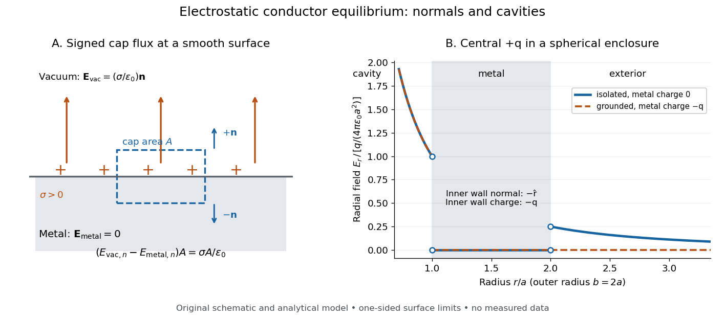
The electrostatic boundary conditions at a conductor relate the one-sided total electric fields at a smooth metal–vacuum interface. Choose a unit normal $\mathbf{n}$ from metal into the adjacent vacuum, let ${\mathbf{E}}_{\mathrm{metal}}$ and ${\mathbf{E}}_{\mathrm{vac}}$ be the two limiting electric fields, and let $\sigma$ be the signed surface charge density. A thin Gaussian pillbox with cap area $A$ has outward cap normals $+\mathbf{n}$ on the vacuum side and $-\mathbf{n}$ on the metal side. As its height tends to zero, its side electric flux tends to zero for bounded local electric fields, leavingThe minus sign comes from the second outward cap normal, not from the sign of the electric charge. A shrinking rectangular loop across the interface and the zero closed line integral in electrostatics give continuity of the tangential component:For a conductor in electrostatic equilibrium, ${\mathbf{E}}_{\mathrm{metal}}=0$, henceThus positive surface charge density gives an electric field away from metal and negative surface charge density gives an electric field toward metal. The derivative uses the same chosen unit normal, from the vacuum side. The ideal surface layer has no unique electric field value on the layer itself; these are limiting values. Ordinary surface electric charge preserves continuity of electric potential; an ideal electric dipole sheet would require a different model. ^[ref].

Here “exterior” means just outside the metal, including the vacuum within a cavity in a conductor. On a spherical inner wall of radius $a$, its unit normal from metal into the cavity in a conductor is $-\hat{\mathbf{r}}$. A central positive point charge $q$ gives ${\mathbf{E}}_{\mathrm{vac}}=q\hat{\mathbf{r}}/(4\pi {ϵ}_0{a}^2)$ there, soThe outward normal of the cavity in a conductor as a volume is instead $+\hat{\mathbf{r}}$; confusing these two unit normals reverses the inferred sign. For a stipulated spherical enclosure with inner radius $a$, outer radius $b$, no external sources and total isolated metal electric charge $Q_c$, spherical symmetry and Gauss's law give the analytical modelIts outer surface charge density is $(Q_c+q)/(4\pi b^2)$. Grounding to $V_c=0$ with zero electric potential at infinity instead gives $Q_c=-q$ and zero exterior electric field, while preserving the same nonzero electric field inside the charged cavity in a conductor.

As a numerical sign check, stipulate $q=1\mathrm{nC}$, $a=0.10\mathrm{m}$, $b=0.20\mathrm{m}$ and $1/(4\pi {ϵ}_0)\simeq 8.99\times 10^9\mathrm{N}{\mathrm{m}}^2/{\mathrm{C}}^2$. The inner electric field is approximately $899N/C$ along $+\hat{\mathbf{r}}$, but ${\mathbf{E}}_{\mathrm{vac}}\cdot \mathbf{n}=-899N/C$ and ${\sigma }_{\mathrm{inner}}\simeq -7.96nC/{\mathrm{m}}^2$. An isolated neutral enclosure has $+1\mathrm{nC}$ on the outer wall, approximately $+1.99nC/{\mathrm{m}}^2$ and $225N/C$ just outside. Multiplying each surface charge density by its spherical surface area recovers the signed wall electric charges.

The local result uses the total electric field, including all induced and imposed sources. The factor $\sigma /{ϵ}_0$ follows from the zero metal-side electric field; a symmetric isolated sheet in vacuum instead has magnitude $|\sigma |/(2{ϵ}_0)$ on each side. ^[ref]. At sharp corners, limiting electric fields can be singular and the smooth local pillbox argument needs care. In material outside the metal, use the normal free-charge jump of the electric displacement field and the material's permittivity, as in electrostatic interface boundary conditions. ^[ref].

A conditional distribution describes the law of a random quantity after specifying information about another. If $Y$ takes values in a measurable space and $X$ is the conditioning variable, a regular conditional distribution is a measurable probability kernel $K(x,A)$ satisfyingfor measurable sets $A,B$. Thus $K(X,A)$ is a version of $\mathbb{P}(Y\in A\mid X)$ for every target event. On standard Borel spaces such kernels exist, and their values are determined only for ${\mathbb{P}}_X$-almost every $x$.

For discrete variables at a point of positive mass, the conditional probability mass function is the familiar joint-mass/marginal-mass ratio. For variables with a joint probability density, the analogous ratio $f_{Y\mid X=x}(y)=f_{X,Y}(x,y)/f_X(x)$ applies where $f_X(x)>0$. When $X$ is continuous, $\mathbb{P}(X=x)=0$ typically holds, so dividing event probabilities by $\mathbb{P}(X=x)$ cannot define the conditional law; the kernel or density construction supplies it instead.

For a bivariate standard normal distribution with correlation $\rho$, the conditional law $Y\mid X=x$ is normal with mean $\rho x$ and variance $1-{\rho }^2$. This shows how an observation changes prediction and remaining uncertainty while the original marginal law of $Y$ remains standard normal.

For a finite measurable partition $(B_j)$ with positive probabilities, and an event $A$ of positive probability,Its beauty is that a model predicting observations from a hidden state can also describe uncertainty about the state after an observation. Each numerator is a joint probability; the denominator, supplied by the law of total probability, makes the answers sum to one. This is a direct consequence of conditional probability, rather than an extra axiom.

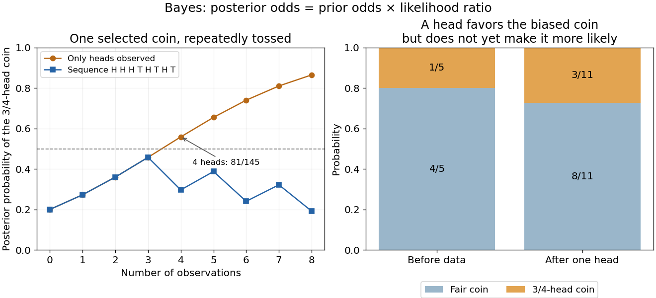
Select the coin from law of total probability once, then toss that same coin repeatedly, with conditionally independent tosses given its identity. Let $B$ denote the $3/4$-head coin, initially of prior probability $1/5$. After one head $H$, its posterior probability isThe likelihood of a head is larger under $B$, but $B$ remains less likely than the other coin because its prior probability was smaller. A large likelihood for an observation does not itself imply a large posterior probability for the hypothesis.

After an ordered sequence containing $h$ heads and $t$ tails, its likelihood ratio between the two coins is $(3/2{)}^h(1/2{)}^t$. Bayes' theorem therefore gives posterior oddsEach head multiplies the odds by $3/2$ and each tail by $1/2$. Three heads give posterior probability $27/59$, still below one half; four give $81/145$, above one half. The finite-model update and the distinction between prior probability, likelihood and posterior probability are set out in MIT 18.05, Reading 11: Bayesian Updating with Discrete Priors.

The hidden selection also creates dependence. Each toss has marginal head probability $11/20$, but two heads have joint probability $(4/5)(1/2{)}^2+(1/5)(3/4{)}^2=5/16$, greater than $(11/20{)}^2=121/400$. Their indicator covariance is $1/100$. Seeing a head makes the head-favoring coin more likely, so it also raises the chance of a future head. This is covariance induced by a shared latent variable, despite conditional independence of the tosses given the coin.

Historically, Thomas Bayes's essay on an unknown success probability appeared in 1763 after his death, communicated by Richard Price. Its opening problem asks how observed successes and failures constrain that unknown probability; Price's introductory letter explains the connection to reasoning from experience. That is a more substantial inference problem than simply rearranging today's elementary identity. ^[ref]

If independent random variables $X,Y$ take values in a finite additive group, thenIndeed, $H(X+Y)\ge H(X+Y\mid Y)=H(X)$, and symmetrically for $Y$. Independence is essential: taking $Y=-X$ makes the sum constant.

For finite discrete random variables $X,Y$, knowing $Y$ reduces the information entropy of $X$ on average:Equality holds exactly when $X$ and $Y$ are independent random variables. The average over observations is essential: $H(X\mid Y=y)$ can exceed $H(X)$ for a particular $y$. All logarithms here have base two, giving bits, and zero-probability terms contribute zero.^[ref]

For Bayesian inference, this compares a prior distribution with the posterior distributions produced by possible observations. An unexpected report can make previously unlikely alternatives plausible, while useful reports reduce uncertainty overall. For lossless source coding, an observation shared by encoder and decoder lets them choose descriptions for the appropriate conditional distribution; sending that observation also has a cost. The example below makes both the saving and that cost explicit.

In A Mathematical Theory of Communication by Claude Shannon (1948), the definition of conditional entropy is already an average over observations, followed by the inequality and its independence condition in section 6, property 6. The phrase “knowledge reduces uncertainty” must be read with that averaging convention.^[ref]

If $f(x,z)$ is a bijection of $x$ for every fixed $z$, thenIn particular, translating a random variable in a finite group by a value determined by the conditioning variable does not change its conditional entropy.

A function is strictly concave when its concavity inequality is strict for distinct points and coefficients strictly between zero and one. A strictly concave function has at most one maximizer on a convex set.

The halting problem asks, given a program and an input, whether running that program on that input eventually stops. It is undecidable: no total algorithm answers correctly for every encoded program and input.

If a decider $H(P,x)$ existed, construct a program $D(P)$ that loops when $H(P,P)$ predicts halting and stops when it predicts nonhalting. Running $D$ on its own description contradicts either prediction. Halting instances are nevertheless computably enumerable, since finite simulations eventually witness any halt. If nonhalting instances were also computably enumerable, dovetailing the two recognizers would decide the problem, so their complement is not enumerable.

If $f(x)=x^{-1/2}g(x)$ with $g$ smooth near zero, the substitution $x=s^2$ givesThe transformed integrand is smooth, so an ordinary second-order midpoint rule recovers its usual convergence rate.

The image of a one-dimensional representation lies in the abelian group ${\mathbb{C}}^{\times }$, so its kernel contains the commutator subgroup of the represented group.