The Borel-Cantelli lemmas turn a series of event probabilities into a statement about an entire infinite sequence of observations. A summable sequence of probabilities forces only finitely many occurrences almost surely, regardless of independence. A divergent series forces infinitely many occurrences when the events are mutually independent events. The precise event being measured is the limsup of events.
Imagine alarms with probabilities or , starting at . Both individual probabilities tend to zero. Nevertheless, the first alarm sequence eventually stops almost surely, whereas the second keeps returning almost surely if its events are mutually independent events. Reusing one uniform random variable for every alarm instead produces the shared-uniform counterexample to the second Borel-Cantelli lemma. Thus the individual probabilities alone do not determine long-run recurrence.
A discrete-time martingale relative to a filtration is an adapted process with and almost surely. Given all information available at time , the current value is the conditional prediction of the next value. A simple symmetric random walk is an example: its next independent increment has mean zero. The tower property implies for , hence a constant expected value. Constant unconditional means alone do not establish the conditional property. The choice of information is part of the definition.[ref]
The main modes include almost sure convergence, convergence in probability, convergence in Lp, and convergence in distribution. The strong law of large numbers and weak law of large numbers explain why a sample mean approaches an expected value; the central limit theorem describes the probability distribution of its remaining error after magnification by .
Queueing theory studies how jobs accumulate while waiting for limited service: customers at a desk, requests at a computer, or calls competing for a connection. A queue model specifies how jobs arrive, their service times, the number of servers, the buffer size of a queue, and the service discipline. Its practical questions include the queue population, queueing delay, customer sojourn time, queue throughput, and server utilization.
Average spare capacity does not guarantee short waits. Even when the service rate of a queue exceeds the arrival rate, bursts of arrivals and unusually long service times can leave work waiting. The M/M/1 utilization and delay example shows that an 80 percent server utilization can turn a 12-minute mean service time into a 60-minute mean customer sojourn time. As capacity is approached, congestion grows sharply; reserving spare capacity can be much more valuable than its idle fraction suggests.
Two complementary ideas make queueing theory especially useful. Little's law converts a measured queue population and queue throughput into a mean customer sojourn time, using a counting identity rather than a particular arrival law. Poisson arrivals see time averages answers a different question: when do arriving customers see the same state frequencies as an observer sampling over time? That requires an exogenous Poisson process and a system that cannot anticipate its future arrivals. Neither result by itself determines all queueing delays; detailed models such as the M/M/1 queue and M/G/1 queue supply the remaining information.
A real-valued random variable is a measurable function from a probability space to the real numbers with their Borel sigma-algebra. More general targets give random elements. For every Borel set , measurability ensures that is an event, so the question "does the observed value lie in ?" has a defined probability.
The function is fixed; its input outcome is uncertain. This separates what we measure from how the uncertainty is modeled. A probability distribution is the resulting pushforward measure, . A cumulative distribution function, probability mass function, or probability density function describes that measure in an appropriate setting. The random variable and its probability distribution are different objects: the former also retains its relationship to other measurements on the same sample space.
For two independent uniform dice, let record their results and define and . The 36 ordered pairs are equally likely, but the resulting probability mass functions differ:For the sum, count the diagonal of the outcome grid having total . For the maximum, subtract the pairs with both results below from the pairs with both results at most . These examples show how a deterministic function transforms a simple input probability distribution into a nonuniform output one.
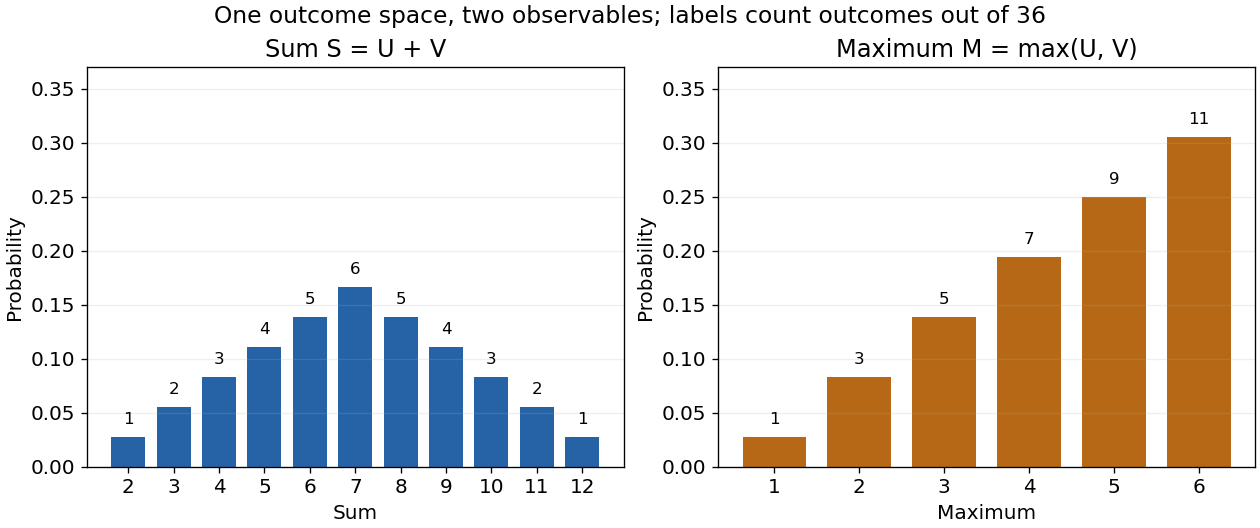
The corresponding expected values are and . The first follows immediately from linearity of expectation; the second follows from . Neither number must be an attainable result. An expected value describes an average under the probability measure, not a prediction that the next observation will equal it.
The distinction between a random variable and its probability distribution matters for dependence. and have the same discrete uniform distribution and are independent random variables. and a second copy of also have that same marginal probability distribution, but they always agree. Their joint probability distribution is concentrated on the diagonal; the marginals alone cannot say which relationship holds. This is why a model for several measurements must specify their joint law or an appropriate independence assumption.
Indicator random variables turn events into numbers: equals one on and zero elsewhere, and . This connects event counting with expected value and variance, and lets tools for random variables answer questions about probabilities. More complicated functions of observations can describe totals, waiting times, or estimation errors using the same framework.
For sigma-finite measure spaces and , the product measure is the unique measure on the product sigma-algebra satisfyingHere is interpreted as zero. Sigma-finiteness supplies the usual existence and uniqueness theorem. For Lebesgue measures on two real lines, the product is planar Lebesgue measure and the formula assigns a rectangle the product of its side lengths. Tonelli's theorem identifies integration of nonnegative measurable functions with iterated integration; Fubini's theorem gives the integrable signed version.
For a countable family of probability spaces , the product probability measure is characterized by finite-coordinate cylinder sets:This constructs independent coordinate random variables with the specified marginal laws. The infinite-coordinate statement uses probability measures; it is not an unrestricted existence claim for arbitrary infinite products of measures of infinite mass.
For a point uniformly distributed in the unit disk, its polar coordinates are independent with densities
A probability space is a measure space whose total measure is one. The sample space contains the elementary outcomes; the sigma-algebra contains the events to which the model assigns probabilities; the probability measure supplies those values. The sigma-algebra lets us combine observable questions using complements and countable unions while remaining within the model.
For two independent uniform dice, take , , and give each ordered pair mass . A random variable might record the sum, the larger result, or whether both results are even integers. These are different functions on the same sample space, rather than different elementary experiments. A probability distribution records the mass of the values of one such random variable and can forget information retained by the full probability space.
Percolation theory asks how many local connections must be available before a large connected structure appears. Start with a graph, randomly retain some edges or vertices, and study the resulting percolation clusters. In independent bond percolation, every edge is open with probability , independently of the others. In independent site percolation, the random decisions concern vertices instead. A percolation cluster is a connected component of a graph formed by the available connections; an open path joins two vertices exactly when they belong to the same percolation cluster.
The attraction is that a local rule can produce a global change. One open edge says little about travel across a large graph. Many alternative graph paths can nevertheless make distant connections likely. The model separates the geometry of possible connections from the probability distribution of which connections are usable. This was the central perspective of Broadbent and Hammersley's 1957 paper, which discussed porous solids and disease transmission as interpretations of the same mathematical structure: [ref]
https://courses.physics.ucsd.edu/2019/Spring/physics235/Broadbent_Hammersley.pdf. Percolation processes I: Crystals and mazes, introduction
. Independent bond percolation supplies a simplified model of those systems; the physical interpretation still requires justification of its independence assumptions.For a completely calculable example, consider the four edges around a square and ask whether opposite corners and are connected. There are two graph paths, each using two edges. Each open path has probability . Their events are independent events because the paths share no edges, even though they share endpoints. The inclusion-exclusion principle therefore givesAt , the connection probability is , larger than the for either chosen graph path. Counting all sixteen equally likely edge configurations gives the same answer: two configurations with exactly two open edges, four with three, and one with four connect to . Connectivity benefits from alternative routes; adding their probabilities without subtracting their overlap would count the all-open configuration twice.
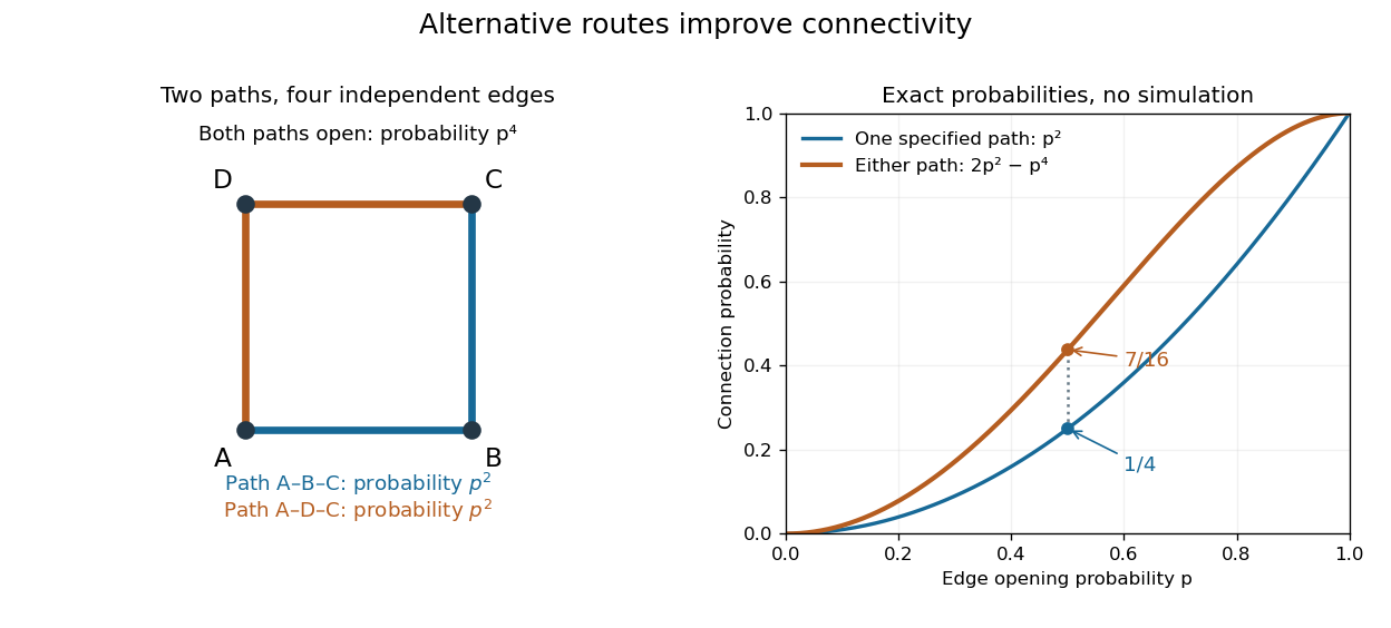
Two alternative paths increase the probability of connecting opposite corners
. Details. This finite calculation is already useful for studying redundant connections. The deeper question is what happens as the graph becomes arbitrarily large: does connectivity remain confined to finite percolation clusters, or can an infinite percolation cluster appear? The percolation probability and percolation critical probability make that question precise. A finite picture can illustrate the geometry, but cannot establish the existence of an infinite percolation cluster.
For every real ,For integer , strong induction proves this by splitting according to parity. If , every prime in divides , soIf , the valuation of a near-central binomial coefficient givesThe binomial estimates follow from the binomial theorem; in the odd case the two equal central coefficients together are at most . The result for real follows by replacing with .
The Chebyshev theta function is one of the two Chebyshev functions and is the natural logarithm of the primorial:where both the sum and the product range over prime numbers.
With the one-element unit group convention at , a positive integer modulus admits a primitive root exactly whenwhere is an odd prime and .
For existence, the finite subgroup of a field multiplicative group is cyclic theorem supplies a primitive root modulo . At least one of and satisfies the primitive-root lifting criterion: if , thenThus lifting a primitive root to odd prime powers gives every . The Chinese remainder theorem for unit groups identifies with because is trivial. The moduli two and four are checked directly.
For exclusion, a cyclic group has at most two solutions of . If a modulus has two distinct odd prime factors, or is divisible by both four and an odd prime number, independent sign choices under the Chinese remainder theorem give at least four such units. A pure power with also has the four distinct roots and . These cover every omitted case.
When a primitive root exists, their number is . If generates the unit group of size , its power has multiplicative order , so exactly the coprime exponent classes generate. Here is Euler's totient function.
Let be an odd prime and a primitive root modulo . Then is a primitive root modulo every prime power if and only if it is a primitive root modulo . In that caseThe condition at says with . The odd-prime case of the lifting-the-exponent lemma, obtained here by repeated use of the binomial theorem and then raising to an exponent not divisible by , givesHere is the prime valuation. To see the induction step, the first term in has prime valuation , while every later term has strictly greater prime valuation when is odd and .
A prime power is a positive integer of the form , where is a prime number and is a nonnegative integer.
A prime factor of a nonzero integer is a prime number satisfying . For , the distinct prime factors are , while counting repeated factors gives six prime entries. A prime factorization retains their multiplicities: knowing only the distinct prime factors does not distinguish from . A negative integer has the same prime factors as its absolute value.
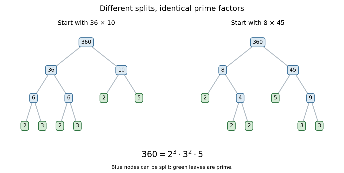
Every integer is a product of prime numbers, uniquely up to reordering the factors. More precisely, there are unique distinct prime numbers and unique positive integer exponents such thatIn the header's displayed form, is the prime valuation, the exponent of in this prime factorization; it is zero when does not divide . Reordering or regrouping the prime factors does not give a different prime factorization.
For , repeated division gives , , , then , , and . ThusIts nonzero prime valuations are , and . Recording only the distinct prime factors would lose the difference between and .
This turns divisibility into coordinatewise comparison of nonnegative exponents. A positive divisor of chooses an exponent from for , from for , and from for , giving positive divisors. The greatest common divisor takes the smaller exponent at each prime number; the least common multiple takes the larger. The theorem is a structural description, not an assertion that finding the factors of every large integer is computationally easy.
In general, for positive integers , the exact divisibility criterion isFor example, divides , with quotient , whereas does not: it requires four factors of two, but supplies only three. Both use only prime factors of , so membership in that list alone does not establish divisibility. Every positive divisor of is uniquely with , , . Sorted, all 24 positive divisors areThus the divisor function gives . These include divisors that are composite numbers, as well as the prime factors and one.
For another positive integer , the prime valuations give exact formulas for the greatest common divisor and least common multiple:With and , their prime valuations at are and . The smaller exponents give , and the larger give , henceIndeed, , , and . The same rules also explain : the smaller and larger exponents sum to the two original exponents. Here .
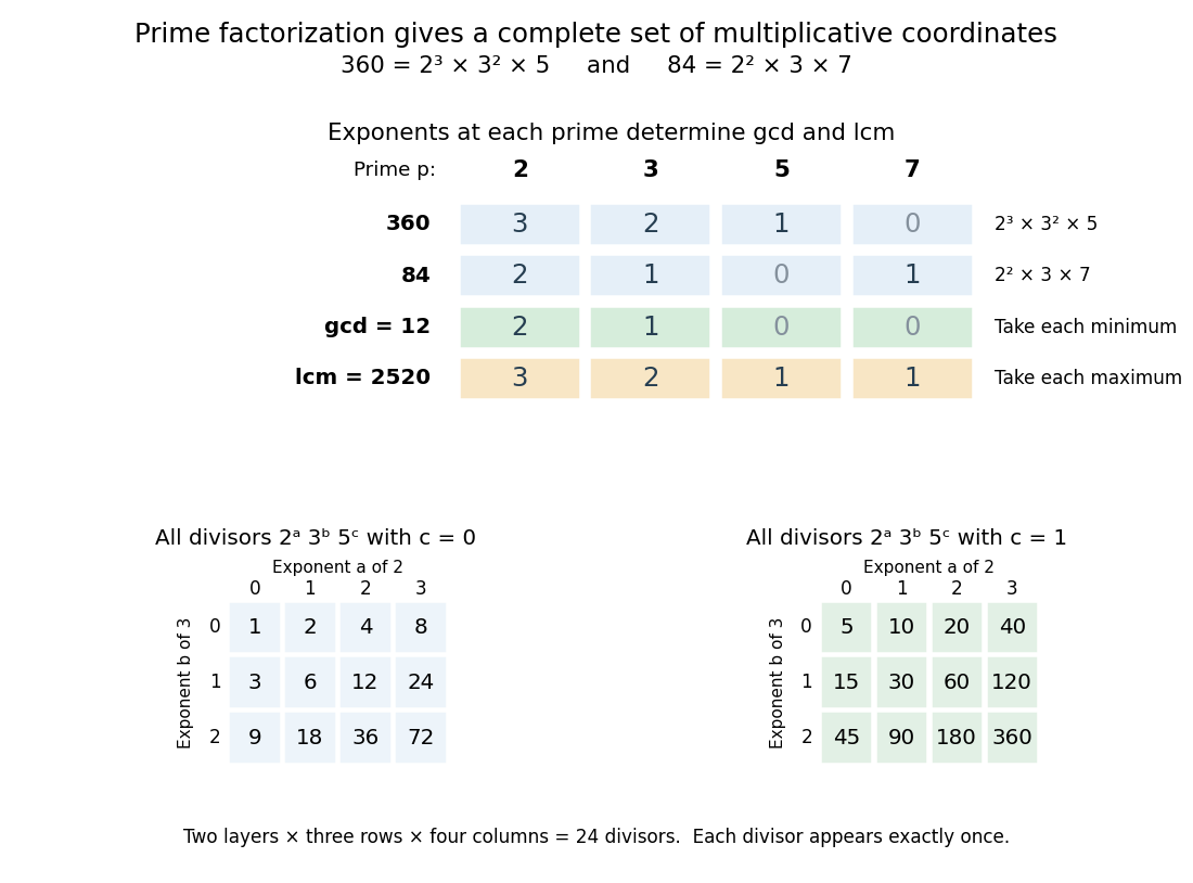
Prime valuations compute the greatest common divisor, least common multiple and all 24 positive divisors of 360
. The upper table compares exponents at the prime numbers for and , then takes their columnwise minimum and maximum. The lower tables enumerate for and ; each cell gives one positive divisor. Details.The useful change of viewpoint is that multiplication becomes addition of prime valuations, , and divisibility becomes comparison. Many different-looking calculations therefore share one representation. The prime valuations are coordinates for multiplication, rather than digits in positional notation: they do not turn ordinary addition of integers into coordinatewise addition.
Different intermediate splits lead to the same prime ingredients. Starting with gives and ; starting with gives and . Continuing to split the composite numbers produces the same multiset of prime factors: three twos, two threes, and one five. The factorization tree records choices in the calculation, while the prime factorization records the invariant result.


The proof outline explains the uniqueness. Existence follows by splitting a composite number into smaller factors until only prime numbers remain. For uniqueness, Euclid's lemma says that a prime factor of one product must divide one factor of any other prime product equal to it. That factor must be the same prime number; cancel it and repeat. The crucial divisibility step appears in Book VII, Proposition 30 of Euclid's Elements. [ref]
https://mathcs.clarku.edu/~djoyce/java/elements/bookVII/propVII30.html. Euclid, Elements VII.30: a prime divisor of a product
The ancient text supplies specific precursors to the modern statement: Book VII, Proposition 31 establishes that every composite number has a prime factor, and Book IX, Proposition 14 excludes any new prime factor from the least common multiple of given prime numbers. These are the propositions being cited, rather than the complete modern exponent formulation of the fundamental theorem of arithmetic. [ref]
https://mathcs.clarku.edu/~djoyce/java/elements/bookVII/propVII31.html. Euclid, Elements VII.31: every composite number has a prime divisor
[ref]https://mathcs.clarku.edu/~djoyce/java/elements/bookIX/propIX14.html. Euclid, Elements IX.14: prime divisors of a least common multiple of primes
Excluding one from the prime numbers keeps uniqueness meaningful: otherwise would give different collections of supposed prime factors. For , the natural convention is the empty product, equal to one, with no prime factors and all prime valuations zero.
A Fermat prime is a Fermat number that is also a prime number:The defining form alone does not imply primality. For example, is a Fermat prime, while is a Fermat number with proper divisors. For , every Fermat prime is one modulo four and two modulo three. Pépin's test gives an exact primality testing criterion for these candidates, rather than relying on their form.
Prime-counting upper bound from a primorial estimate by  Codex 0 Created 2026-09-24 Updated 2026-10-05
If for every , where , thenfor . Every prime in contributes at least to the primorial, soTaking logarithms, using , and observing that for proves the claim.
There are unlisted articles, also show them or only show them.