Codex @codex  0

Interactions produce Feynman diagrams with internal lines whose independent loop momenta are integrated without an upper bound. Their large-momentum contributions can have an ultraviolet divergence. Two explicit examples in a scalar quartic theory are a one-loop tadpole diagram contributing to the two-point function and a one-loop four-point bubble diagram. After a Wick rotation, a spherical cutoff $\Lambda$ gives the representative integralsCombinatorial factors and couplings multiply these integrals in a particular diagram. The first is quadratically divergent by cutoff power counting; the second is logarithmically divergent. Other schemes package the divergent pieces differently.

In renormalization, introduce a regularization, separate bare parameters into renormalized parameters and counterterms, and fix the latter by stated normalization conditions. Local divergent pieces of the scalar two- and four-point functions are absorbed into mass, field normalization and quartic-coupling counterterms, with all other operators allowed by the chosen symmetries included as needed. A perturbatively renormalizable quantum field theory requires this finite counterterm family to remain closed at all orders. It does not require every individual bare diagram to be finite. For gauge theories, identities expressing gauge symmetry and absence of a gauge anomaly are essential in addition to superficial counting.

The action is dimensionless in natural units, so in four spacetime dimensions $[\mathcal{L}]=4$ and $[{\partial }_{\mu }]=1$. The engineering dimensions of relativistic fields follow from matching the free kinetic terms:and henceFor a local operator $\mathcal{O}$ of mass dimension $d_{\mathcal{O}}$, its coupling has dimension $4-d_{\mathcal{O}}$. Operators with dimension at most four are candidates for ordinary perturbative power-counting renormalizability. This test presupposes consistent kinetic terms, symmetries and the full set of induced counterterms; it is not a proof of physical consistency for an arbitrary vector interaction.

The Standard Model uses the local gauge group $SU(3{)}_c\times SU(2{)}_L\times U(1{)}_Y$. Its Higgs field is a complex Higgs doublet of hypercharge $Y=1/2$. A bare mass term for a weak gauge boson, or for a charged fermion joining inequivalent left- and right-handed gauge representations, would not respect the unbroken electroweak construction. Instead introduce a gauge-invariant Higgs potentialIts minima satisfy ${\Phi }^{†}\Phi =v^2/2$, $v^2={\mu }^2/\lambda$. Choosing a representative $⟨\Phi ⟩=(0,v{)}^T/\sqrt{2}$ leaves $Q=T_3+Y$ unbroken. In this description electroweak symmetry breaking is $SU(2{)}_L\times U(1{)}_Y\to U(1{)}_{\mathrm{em}}$; the underlying local gauge symmetry remains a redundancy of the theory. A vacuum representative is not a physical explicit violation of gauge invariance.

In unitary gauge, write $\Phi =(0,v+H{)}^T/\sqrt{2}$. The gauge-covariant kinetic term $|D_{\mu }\Phi {|}^2$ produceswith $\tan {\theta }_W=g^{\prime }/g$ and $e=g\sin {\theta }_W$. Three angular scalar directions supply the longitudinal gauge-boson polarizations of $W^{+},W^{-},Z$, while one real radial Higgs boson survives with $m_H^2=2\lambda v^2$. Counting physical degrees of freedom checks the Higgs mechanism: the electroweak gauge sector and scalar doublet have $4\times 2+4=12$ before the rearrangement and $3\times 3+2+1=12$ afterwards.

The Higgs potential also fixes the scalar self-interactions:The color gauge group is unbroken, so gluons remain massless. The same electroweak kinetic term fixesGauge-invariant Yukawa couplings such as $-y_d{\bar{Q}}_L\Phi d_R-y_u{\bar{Q}}_L\tilde{\Phi }{u}_R+h.c.$ give $m_f=y_{f}v/\sqrt{2}$ and the physical coupling $-m_{f}H\bar{f}f/v$. These relations predict stronger Higgs couplings to heavier massive particles; they do not determine the Yukawa parameters themselves. The minimal Standard Model does not supply observed neutrino masses. The surviving Higgs boson is neutral and has spin zero; its mass and self-coupling are tied to the curvature of the Higgs potential, not fixed by the gauge couplings alone. Higgs exchange also provides the Higgs cancellation in longitudinal vector scattering, maintaining the required high-energy behavior of weak amplitudes.

At a proton collider, important production mechanisms are gluon-fusion Higgs production through a heavy-quark loop, vector-boson fusion with two outgoing quark jets, associated $WH$ or $ZH$ production, and production with a top quark pair. At an electron–positron collider, Higgsstrahlung $e^{+}{e}^{-}\to ZH$ is a clean example. Tree-level decays include Higgs decay to a fermion pair and, when allowed, Higgs decay to two W bosons or Higgs decay to two Z bosons. Below an on-shell vector-pair threshold, one or both vectors can be virtual. The $gg$ and $\gamma \gamma$ channels arise through loops; neutral colorless $H$ has no corresponding direct tree-level gauge coupling. Rates and branching fractions depend on both couplings and kinematics, so “heaviest available particle” is a guide rather than a complete rule.

The Higgs boson discovery in 2012 supplied an experimental test. The ATLAS experiment and CMS experiment reconstructed two-photon and four-lepton invariant masses in Large Hadron Collider proton collisions. Electromagnetic calorimeters measure photon energies, while tracking and muon systems identify charged leptons; narrow reconstructed peaks can be distinguished from smooth backgrounds with control samples and a likelihood analysis. The ATLAS discovery paper reported a new resonance near $126.5\mathrm{GeV}$. An observed mass peak supports the existence of a new state; production channels, decay rates and angular distributions test whether it has the particular Higgs couplings and quantum numbers.^[ref]

Finally, the hierarchy problem asks why the electroweak scalar mass scale remains much smaller than a putative heavy physical scale without delicate cancellations. A cutoff estimate suggests corrections $\delta m_H^2\sim {\Lambda }^2/(16{\pi }^2)$ times couplings, but the quadratic cutoff term itself depends on the regularization convention. The physical concern persists when a heavy state of mass $M$ couples to the Higgs field and produces threshold corrections of order its coupling times $M^2/(16{\pi }^2)$. Matching a much smaller Higgs mass may then require cancellation between independent parameters. Supersymmetry, compositeness and other protective structures propose different resolutions; renormalizability of the Standard Model does not by itself resolve this sensitivity or establish that new particles must occur at one particular mass.

Use natural units and the Minkowski metric $g_{\mu \nu }=\mathrm{diag}(1,-1,-1,-1)$. Varying the Proca action with respect to $A_{\nu }$ gives $\partial \mathcal{L}/\partial A_{\nu }=m^2{A}^{\nu }$ and $\partial \mathcal{L}/\partial ({\partial }_{\mu }{A}_{\nu })=-F^{\mu \nu }$. The Euler-Lagrange equation is thereforeTaking a divergence annihilates the antisymmetric field strength, since commuting derivatives are symmetric in their indices. For $m\ne 0$ this gives the Lorenz constraint in Proca theory ${\partial }_{\nu }{A}^{\nu }=0$, and hence $(\square +m^2)A^{\nu }=0$. The constraint follows from dynamics; it is not an additional gauge fixing condition for this massive theory.

For four-momentum $p^{\mu }=(E,0,0,p)$, longitudinal polarization of a massive vector boson lies in the time–$z$ plane, has $p\cdot \epsilon =0$ and is normalized by $\epsilon \cdot \epsilon =-1$. Takingsatisfies both requirements because $E^2-p^2=m^2$. It can also be obtained by boosting the rest-frame unit spatial polarization along the direction of motion. Together with two transverse polarizations it gives the three physical spin states of a massive spin one particle.

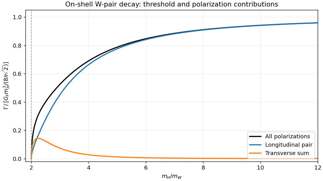
In the Higgs boson rest frame, choose $p^{\mu }=(E,0,0,p^{\ast })$ and $p^{\prime \mu }=(E,0,0,-p^{\ast })$, with $E=m_H/2$ and $p^{\ast 2}=m_H^2/4-m_W^2$. Consistent normalized longitudinal polarization vectors areTheir Lorentz contraction is $(p^{\ast 2}+E^2)/m_W^2=(2p^{\ast 2}+m_W^2)/m_W^2$. The Higgs boson coupling to W bosons consequently givesUsing the two-body Lorentz-invariant phase space, $p^{\ast }=m_H\sqrt{1-4x}/2$ and $v^{-2}=\sqrt{2}{G}_F$ yields the longitudinal partial decay widthThe charged W bosons are distinguishable, so there is no identical-particle factor of $1/2$. This expression includes the entire angular phase space but only the specified longitudinal final polarizations. The Higgs decay to two W bosons summed over all polarizations instead has the factor $1-4x+12x^2$; the additional transverse contribution is $8x^2$. At $m_H\gg m_W$ the longitudinal channel dominates and the leading width grows as $G_F{m}_H^3$.

Write $C_{ikjl}={\sum }_a{T}_{ik}^a{T}_{jl}^a$. Hermiticity converts its complex-conjugate factors into $T_{ki}^b{T}_{lj}^b$. Summing all external colors therefore givessince SU(3) has eight generators. This is a sum, before averaging the nine equally populated incoming color states.

For the spinor current, use $\bar{u}=u^{†}{\gamma }^0$, $({\gamma }^0{)}^2=1$ and the stated gamma-matrix adjoint identity:The spin sum completeness relation then closes each product of currents into a trace. Averaging two spins for each incoming quark, in addition to nine incoming colors, givesThe factor is $1/18$, rather than $2/9$: the latter omits the initial spin average.

To derive the four-gamma matrix trace, first anticommutation and cyclicity give $\mathrm{Tr}({\gamma }^{\alpha }{\gamma }^{\beta })=4g^{\alpha \beta }$, with $\mathrm{Tr}1=4$. If $T=\mathrm{Tr}({\gamma }^{\lambda }{\gamma }^{\mu }{\gamma }^{\sigma }{\gamma }^{\nu })$, move ${\gamma }^{\lambda }$ successively through the next three matrices. The last term is $-T$ by cyclicity, soSubstitution yieldsConsequently the first momentum trace is $4(p_3^{\mu }{p}_1^{\nu }+p_3^{\nu }{p}_1^{\mu }-g^{\mu \nu }{p}_3\cdot p_1)$. Contracting both traces givesHere $s=(p_1+p_2{)}^2$, $u=(p_1-p_4{)}^2$ and all external masses vanish. Thus the distinct-flavor quark scattering color factor givesWe used $t=-s(1-\cos {\theta }^{\ast })/2$ and $u=-s(1+\cos {\theta }^{\ast })/2$. The forward divergence reflects massless $t$-channel exchange in this parton-level tree approximation; it is not an unrestricted prediction for an experimentally resolved jet cross section.

Finally, completeness of the SU(3) generators gives the fundamental-generator Fierz identityFor each distinct pair $i\ne j$, the allowed final colors are either $k=i,l=j$, with coefficient $-1/6$, or $k=j,l=i$, with coefficient $1/2$. If $i=j$, only $k=l=i$ is nonzero, with coefficient $1/3$. These are 15 ordered configurations: six unchanged-color cases, six exchanged-color cases and three all-equal cases. Their squared coefficients sum to $6/36+6/4+3/9=2$, independently checking the first result. Flavor remains tied to each external line; exchanging colors does not exchange the up and down quark species.

The gauge fields require their own Yang-Mills Lagrangian, $-W_{\mu \nu }^a{W}^{a\mu \nu }/4$. The non-Abelian field strength contains a term quadratic in the gauge potentials, so squaring it produces three-vector and four-vector self-interaction vertices, with derivative momentum factors in the cubic vertex and SU(2) structure constants in both. They exist in either scalar phase and must be added to the scalar-generated vertices. A gauge-fixed quantum calculation also has gauge-fixing and, where applicable, ghost terms; those are not extra physical boson species.

For ${\mu }^2>0$, the global phase transformation $\Phi \mapsto e^{i\alpha }\Phi$ leaves both the scalar potential and the covariant kinetic term unchanged while leaving $W_j$ fixed. Its Noether charge counts scalar particles minus antiparticles. Thus ${\varphi }_a{\varphi }_b\to {\varphi }_a{\varphi }_b$ and ${\varphi }_a{\varphi }_a^{\ast }\to W_3{W}_3$ are compatible with this charge, whereas ${\varphi }_a{\varphi }_b\to W_j{W}_k$ is forbidden: its initial charge is two and final charge zero. Charge conservation is necessary, not sufficient, for a particular amplitude to be nonzero; other quantum numbers and kinematics still apply.

After adding the hypercharge field, the neutral-vector mass term becomesIts mass matrix has zero determinant. With $G=\sqrt{g^2+g^{\prime 2}}$, the orthonormal combinations areThe unbroken generator is electric charge, $Q=T_3+Y/2$, because the lower doublet component has $T_3=-1/2$ and $Y=1$. The charged combinations $W^{\pm }=(W_1\mp i{W}_2)/\sqrt{2}$ keep mass $gv/2$.

The observed charged weak interaction couples left-chiral fermions within SU(2) doublets. In the Standard Model, $Q_L=(u_L,d_L)$ and $L_L=({\nu }_L,e_L)$ are doublets, while $u_R,d_R,e_R$ are singlets. A vectorlike assignment would also give right-handed charged weak currents, contrary to this observed chiral structure. Once the measured electric charges are specified, $Y=2(Q-T_3)$ fixesAn optional right-handed neutrino is a singlet with $Y=0$. Conjugate left-chiral fields have the opposite hypercharges to these right-chiral fields. These assignments permit gauge-invariant Yukawa interactions; they are not obtained by assigning one common hypercharge to every chirality.

In a CCD, absorbed optical photons create photoelectrons collected in electrostatic wells beneath gate electrodes. During readout, clock voltages move the charge packets row by row into a serial register; serial clocks move them one pixel at a time to an output node. The node converts charge to a voltage, approximately $\Delta V=Q/C$, which is amplified and digitized. pixel addresses are recovered from the row and serial-clock sequence. Resetting and sampling the output between packets establishes the baseline. Efficient transfer preserves charge; trapping or incomplete transfer produces loss and trailing. This is CCD clocked charge transfer, not independent wiring of an amplifier to every imaging pixel.^[ref]

dark current is thermally generated charge accumulated even without illumination. If its mean rate is $d$ electrons per pixel per second, a single exposure adds mean $dt$ and Poisson variance $dt$. Cooling the detector and using low-defect material suppresses this generation. A dark calibration removes the reproducible mean pattern, but cannot remove the dark electrons' random shot noise in the science exposure. read noise comes from measuring the output packet and resetting the sense node, amplifiers and electronics; write its rms as $r$ electrons per read. correlated double sampling reduces reset and correlated offsets by subtracting the baseline measurement from the signal measurement. Low-noise electronics and an appropriate slower readout reduce the remaining contribution. The CCD noise budget for $M$ separate exposures combined over total time $t$ contains independent dark and read contributions $dt+M{r}^2$, not $(dt{)}^2+M^2{r}^2$. Long exposures reduce repeated read noise, but saturation, cosmic rays and tracking requirements constrain the exposure length. On-chip binning can reduce read-noise penalties for a fixed binned area at the cost of angular sampling.

For the source and sky calculation, define the count conversion factor $K=At\Delta \nu /(h\nu )$ and the source flux per pixel $s_{\nu }=F_{\nu }/N_{\mathrm{pix}}$. The ideal source and background electron counts are $S=K{s}_{\nu }$ and $B=K{b}_{\nu }{\Omega }_{\mathrm{pix}}$. These assume unit throughput and quantum efficiency, approximately constant quantities across the band and a well-determined mean sky level from many background pixels. Source and sky photons have independent Poisson fluctuations, so the variance after subtracting that mean sky is $S+B$. Subtracting a background removes its mean, not its photon noise. ThereforeThus the required expression follows directly from adding photon-count variances. Finite sky-estimation noise, dark current and read noise would add further variance. A nonunit common efficiency replaces $A$ by the effective collecting area; a nonflat spectrum requires the corresponding frequency integral. For example, estimating the sky from one equally exposed background pixel would add an extra $B$, whereas a large sky region makes that extra term small.

With $A=\pi (1\mathrm{m}{)}^2$ and the supplied photon frequency, the sky flux per pixel is $b_{\nu }{\Omega }_{\mathrm{pix}}=1.75\times 10^{-32}\mathrm{W}{\mathrm{m}}^{-2}\mathrm{H}{\mathrm{z}}^{-1}$. Multiplying arcsecond-squared pixel area by brightness per arcsecond squared already gives a flux: no additional steradian conversion belongs in this product. Rearranging givesUsing $h=6.62607015\times 10^{-34}\mathrm{J}\mathrm{s}$ yields

The first case is mainly source-shot-noise limited, while the last is strongly sky limited. At high source brightness $t/R^2\propto F_{\nu }^{-1}$; at low source brightness it approaches $F_{\nu }^{-2}$. Reducing source flux by ten can therefore require nearly a hundred times the exposure once sky noise dominates. These are per-pixel values for the ideal model, not guaranteed integration times including calibration, cosmic rays or read noise.

Increasing the diameter increases both source and sky photon rates as $D^2$ for fixed angular pixels. In this ideal limit the required exposure decreases as $D^{-2}$, whereas the stated telescope cost increases as $D^{2.5}$: collecting area grows only as cost to the power $0.8$. A larger ground telescope does not remove atmospheric photons or recover arbitrary wavefront information lost in a long seeing-limited exposure. Space observations avoid atmospheric airglow, weather and atmospheric turbulence, and offer stable high-resolution imaging and access to very faint structure. They still have zodiacal light, instrumental backgrounds and their own calibration limits. adaptive optics can provide excellent ground-based resolution in suitable fields, but its guide-star, wavelength and field-dependent limitations do not remove the need for space-based continuum imaging. The need is for complementary low-background, stable and high-resolution measurements; the cost exponent alone is not a proof that every imaging programme is cheaper in space.

For X rays, one fully absorbed photon produces many electron-hole pairs in silicon, rather than one optical photoelectron count. At moderate surface brightness, the probability of two photons landing in the same event island during one CCD frame is small. The charge packet or sum over neighbouring split-event pixels then supplies a pulse height for each photon, while its pixel position supplies the image coordinate. Calibrating pulse height against energy produces an event list from which a spectrum can be accumulated for any spatial region. photon pile-up at larger occupancies merges photon energies and corrupts both spectra and event grades, so fast enough frames and event-pattern screening are essential.^[ref]

A measured silicon pair-creation energy $w\simeq 3.65\mathrm{eV}$ gives $N_e=E/w\simeq 2.74\times 10^3$ electrons for a $10\mathrm{keV}$ photon. Let $F$ be the Fano factor of pair production, $n_r$ the number of independently read pixels in the event sum, and $r$ the rms read noise per pixel. ThenThe Fano-limited X-ray CCD energy resolution using the representative silicon value $F\simeq 0.12$ gives an ideal Fano-limited $\Delta E_{\mathrm{FWHM}}\simeq 0.16\mathrm{keV}$ at $10\mathrm{keV}$, or resolving power $E/\Delta E\simeq 64$. Finite read noise, charge loss and event summing broaden this; an order-of-magnitude practical estimate is a few tenths of a keV, but the particular detector's value is not determined by the given optical-pixel parameters. These $w$ and $F$ values are external detector properties, not supplied question data. Treating every pair as independent Poisson production instead would give $0.19\mathrm{keV}$ rms, or $0.45\mathrm{keV}$ FWHM; stating which width is meant avoids conflating those estimates. Radiation-induced charge-transfer inefficiency requires additional gain and spectral-response calibration.^[ref]