
For a real function bounded by one on a finite Cartesian product, the fourth power of its box norm is the mean of . Two applications of the Cauchy-Schwarz inequality bound every rectangular discrepancy by the box norm. Conversely, decompose each bounded real test function into positive and negative parts and use the layer cake representation. Its bilinear pairing with is at most four times the cut norm. Applying this to the row and column tests furnished by fixed bounds the fourth moment by four times the cut norm. These dimension-independent estimates make the two notions of small discrepancy equivalent.
Give every entry of an by matrix an independent uniformly random sign. A four-entry rectangle product has expectation zero unless its two row indices coincide or its two column indices coincide; in those cases it is one. Counting the union of these diagonal cases gives before normalization. Thus some sign matrix has box norm fourth power at most the displayed expectation, and its cut norm tends to zero when both dimensions tend to infinity.
Consider base- expansions using allowed digits with positive gaps between the corresponding first-level intervals. At depth there are cylinders of diameter comparable to , and separated cylinders cannot all be covered by fewer than a constant multiple of balls of that scale. Thus . Monotonicity between successive scales gives equal upper and lower Minkowski dimensions, both .
Uniformly stratified, nonrotating, two-dimensional ideal Boussinesq equations in coordinates are equivalent to unstratified rotating equations independent of , with , rotation , velocity , and the same reduced pressure. The transverse rotating velocity represents buoyancy perturbation, while the rotation-axis velocity represents the stratified horizontal velocity. Matching prescribed forces may have components in the invariant plane, but no transverse component. Physical free surface conditions are not preserved: the physical vertical direction and its normal velocity are different under the mapping.
In the constant-property convection convention, the strong Boussinesq approximation supplements small relative mass density changes with constant dynamic viscosity, thermal diffusivity, specific heat capacity and thermal expansion coefficient throughout the modeled temperature interval. A uniform reference density replaces density in inertia and mass conservation, while a linear density anomaly is retained in gravitational buoyancy. The temperature obeys an advection-diffusion equation with constant coefficients. The term “strong” is not uniform across all fluid-mechanics literature: some stratified-flow treatments instead emphasize the use of a globally constant reference density. The constant-property convection usage is explained in courses.physics.ucsd.edu/2021/Spring/physics218c/Spiegel%20Convection.pdf .
The momentum thickness weights the streamwise velocity deficit by the local velocity carrying it:Thus measures a momentum flux deficit per unit span relative to transporting the same local mass flow rate at . It is not , which compares a different reference flux. A Blasius boundary layer has ; the ratio of displacement thickness to momentum thickness is about .[ref]
For the steady flow over an impermeable flat plate at constant , integrating the boundary-layer equation and using mass conservation givesThis connects growth of the momentum thickness to local wall shear stress. Consequently the drag per unit span on one face up to is in the ideal Blasius boundary layer with . Measured velocity profiles can therefore estimate integrated drag without differentiating noisy near-wall readings. The identity assumes no wall suction and zero outer pressure gradient.[ref]
For constant-mass density incompressible flow, the displacement thickness measures the lost volume flux per unit span divided by the outer velocity:An outer inviscid flow encountering the same volume flux deficit behaves, at leading order, as though the wall were displaced outward by . In a Blasius boundary layer, numerical integration gives . This equivalent displacement is smaller than the boundary layer thickness and is not the position of a physical surface.[ref]
A cover of by closed sets has a member containing an antipodal pair. The equivalent version for open sets follows by shrinking finite open covers on a compact metric space; the reverse implication follows by enlarging antipodal-pair-free closed sets slightly. This is a covering formulation of the Borsuk-Ulam theorem.
A second indirect route makes the experimental distinction especially clear: a calorimeter can measure dissolution of a weighed salt into a known amount of water, but its final ions are hydrated, not separated gaseous ions. At compatible standard states and the same temperature,Here the combined hydration of ions term takes one mole each of gaseous and to the specified aqueous reference state. Its sum suffices: dissolution calorimetry alone cannot independently assign single-ion hydration of ions enthalpies, or determine without another input. A finite-concentration measurement also requires dilution corrections before it can supply .
In a simple constant-pressure solution calorimeter, an insulated vessel, stirrer and thermometer follow the temperature change after mixing. A calibrated effective heat capacity converts the corrected temperature change to heat. With no applied heating, negligible external heat transfer, and only pressure-volume work, the approximate molar result isHere is the amount of substance dissolved and includes the chemical solution and the vessel. Cooling means positive dissolution enthalpy, because the dissolving sample takes heat from its surroundings.[ref]
Chemistry 2e. §5.2, Figures 5.11–5.13 and discussion of including solution and calorimeter heat capacities
An actual reference measurement used potassium chloride, not sodium chloride: a platinum-lined calorimeter with an adiabatic shield and a quartz-oscillator thermometer. Because dissolution absorbed heat, measured electrical heating prevented loss of shield control; the readouts were electrical input and the vessel/shield temperature record. Stirring was checked visually in a dummy vessel. The thermometer was compared with a calibrated resistance thermometer, and electrical calibration bracketed the reaction. The reported result was at , for one mole of potassium chloride in moles of water.[ref]
The Enthalpy of Solution of SRM 1655 (KCl) in H2O by Marthada V. Kilday. §3 and §4: apparatus, calibration, readouts and specified dilution; inspected through indexed article text
Checks on residual water, particle size and final concentration, and agreement with a second calorimeter, constrained systematic errors. Imperfect shield tracking required heat transfer corrections. This experiment measures an enthalpy of solution, not a direct lattice energy; the hydration and dilution bookkeeping still has to be supplied. The full article could not be opened here; the inspected indexed text supports the stated apparatus and checks, without reconstructing its complete uncertainty budget.[ref]
The Enthalpy of Solution of SRM 1655 (KCl) in H2O by Marthada V. Kilday. §§2–4 and conclusion: moisture, particle-size and dilution studies; confirmation with an isoperibol calorimeter; full-page access blocked
Removing factorial growth from the coefficients of a formal inverse-power series produces its Borel transform. When continuation and exponential growth bounds allow it, reconstructs the series by Laplace transform. A singularity on the integration direction requires a lateral contour prescription. A simple pole contributes a residue when that prescription is changed, explaining how Stokes phenomenon arises from otherwise identical algebraic expansions.
If the events are mutually independent events and , then . For an infinite family, mutual independence means every finite subfamily satisfies the factorization defining independent events.[ref]
Proof outline: for , independent events and giveContinuity of probability makes each infinite tail union have probability one; their countable intersection has probability one as well.
For independent standard normal random variables , the displayed limit superior equals two almost surely. The Mills ratio asymptotic gives, for ,The series converges for and diverges for . The two Borel-Cantelli lemmas, applied at countably many thresholds approaching two, give the result. In particular, the value two is also a threshold exceeded infinitely often, despite being the almost-sure limit superior.
Take independent random variables , each with the continuous uniform distribution on , and set . Then , and the events are mutually independent events. The product probability space supplies a model for the entire infinite sequence; a finite list of simulated values is only an illustration.
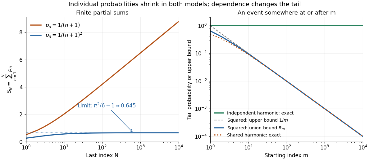
For , the p-series is summable:The Basel problem supplies the total sum, and the integral test for convergence gives the displayed tail bound. The First Borel-Cantelli lemma makes the limsup of events have probability zero. In fact, the tail bound implies that the probability of even one alarm at or after is at most ; for , it is at most . This bound remains valid for dependent events with the same individual probabilities.
For , the harmonic series diverges, so the Second Borel-Cantelli lemma makes the limsup of events have probability one. There is also an exact finite-horizon calculation using independent events:For any fixed , this finite product of numbers tends to zero as . Every infinite tail therefore contains an alarm almost surely, even though the individual probabilities tend to zero.
Circuit depth is the largest number of counted gates on any input-to-output path in the Boolean circuit. For an AND/OR circuit with negations on input literals, only the AND/OR gates are counted. This convention makes the restriction argument for the Linial-Mansour-Nisan theorem precise.
The size of a Boolean circuit counts its gates, or in another common convention its wires. The convention must be fixed when stating quantitative bounds. In switching arguments, new clauses created from a decision tree are not separate original gates to be charged in the failure union bound.
For the number of occurring events, write and . Then odd truncations bound below and even truncations above. For each integer , the truncated binomial sum equals when , and is zero otherwise. Its sign proves the bounds on taking expectations. This is the exact-count version of the Bonferroni inequalities.
For the normalized isotropic Maxwell molecule collision operator, put and . The integral is over position, both velocities and collision direction. The symmetrized weak identity yields the displayed derivative of the Boltzmann H functional. It is nonpositive because for positive . Spatial transport contributes only a boundary flux, which must vanish for the total-space inequality.
Keep the gap fixed and vary positive temperature. With , the Boltzmann factor is . In the four-microstate example, as , : the unique ground state has probability tending to one, and the other microstates have probabilities tending to zero. If several microstates instead shared the lowest energy, their state degeneracy would split that limiting population equally.
As in this fixed finite model, all four individual Boltzmann factors tend to one, so all four individual microstates have probability tending to . The three aggregate probabilities instead approachThe equal-population limit applies to this finite set of microstates. An infinite collection of microstates cannot all have the same positive normalized probability, so the statement cannot be extended to an unbounded energy spectrum. Real systems may also acquire additional accessible microstates as temperature rises.
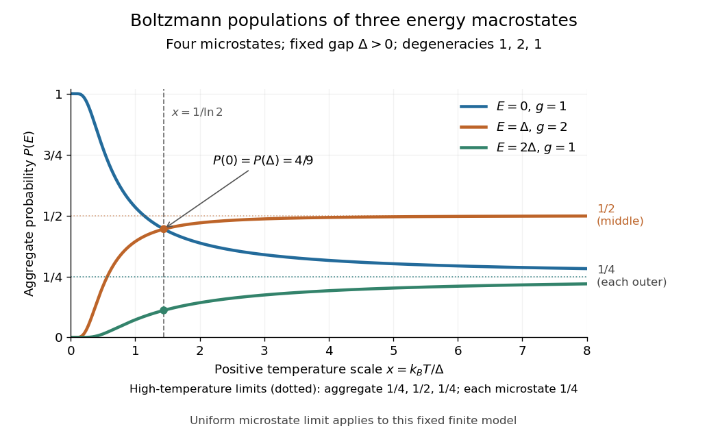
Aggregate Boltzmann distribution populations versus positive temperature for state degeneracies 1, 2, 1
. Details. The plotted crossing occurs at , where . For larger positive temperatures, the middle macrostate is more probable than the lowest-energy macrostate, although the lowest-energy individual microstate remains more probable than either individual middle microstate. The expected value of energy rises from zero toward in this finite model.
Consider two distinguishable, noninteracting two-level systems, each with energies and . Their four microstates have total energies . Thus the three energy macrostates have state degeneracies . This is a stipulated finite model, not a measured material.
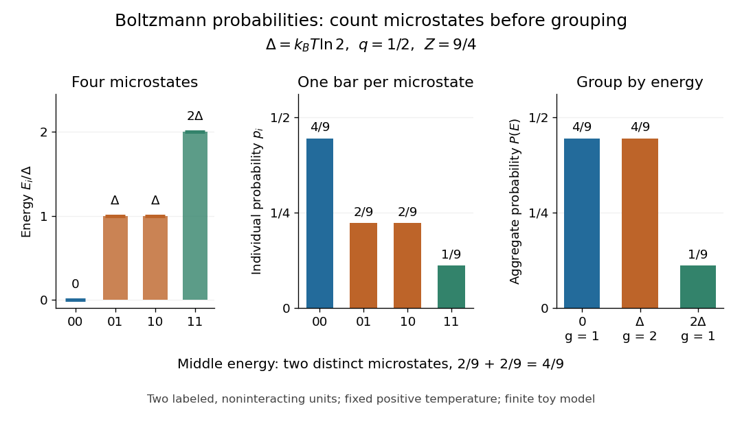
Set . The four individual Boltzmann factors are , so the partition function and aggregate probabilities areEach of the two middle microstates has probability , while their shared energy macrostate has probability .
At the temperature satisfying , the Boltzmann factor is and the partition function is . ThereforeThe middle energy is as likely as the ground state energy because its state degeneracy is twice as large. Yet each individual middle microstate is only half as likely as the ground state microstate. The diagram places the four energies beside their individual probabilities, then shows the sums within each macrostate.


The expected value of energy follows directly by weighting the three possible energies:At this is . An individual energy measurement still returns , or ; the expected value describes the ensemble average, rather than a fourth possible measured energy.
Group microstates by their energy . The state degeneracy counts how many microstates have that energy; their aggregate probability isHere is the probability of the macrostate retaining only energy, while is the probability of one individual microstate. For two such macrostates,Counting more microstates can compensate for a smaller Boltzmann factor. Omitting the state degeneracy confuses a sum over microstates with a sum over distinct energies. [ref]
https://ocw.mit.edu/courses/5-62-physical-chemistry-ii-spring-2008/bda82786b6014d3f468798339f658629_03_562ln08.pdf. MIT 5.62, spring 2008, lecture 3, page 4: degeneracy and the aggregate energy probability
There are unlisted articles, also show them or only show them.