
These bounded-unitary relations encode a pair of canonical commutation relations without multiplying unbounded position and momentum operators. In a fixed convention on , and . Strong continuity is part of a regular Weyl representation. Different nonzero choices of the central normalization rescale the canonical coordinates.
A calorimeter infers transferred heat from a measured change, such as a temperature change and a calibrated heat capacity. The heat-engine calorimetry example requires accounting for the vessel and heat transfer to the surroundings as well as the water.
A practical receiver has an inner vessel, insulation or an outer shield, a lid, a thermometer and a stirrer. Its participating heat capacity includes the immersed parts that follow the water's temperature. Insulation reduces heat transfer to the room; stirring makes a single reading more representative of the contents. These serve different purposes: a well-insulated vessel can still have substantial heat capacity, and a uniform temperature does not imply zero external heat transfer.
The University of Toronto's Heat Capacity (University of Toronto laboratory handout) describes a copper inner vessel, outer shield, thermometer and heated metal block. Weigh the block and receiving water, heat the block in a bath, then transfer it quickly into enough water to cover it. The observed temperature rises, reaches a maximum, then falls. The inferred specific heat capacity comes from the block's cooling and the warming of both water and vessel. In its cooling exercise the handout deliberately exposes the inner vessel to room air, recommends readings every , and uses the later common cooling to estimate the earlier loss. Starting below room temperature reduces exchange without guaranteeing cancellation. The handout notes limited time and thermometry for small corrections; it supplies no dataset.[ref]
Heat Capacity (University of Toronto laboratory handout). pp. 1–3, The Method of Mixtures and Cooling Correction, Figure 1
For a proposed modern version, independently perform thermometer calibration and calorimeter calibration, record bath and room temperatures, and keep immersion depth, lid position and stirring rate fixed. Ensure the block actually reaches bath temperature; minimize and account for adhering hot bath water. Compare repeated transfers with different delays and a reference sample of known specific heat capacity. A resting run tests environmental heat transfer, while a stirred run with no added sample checks mechanical input. These are proposed controls, not claimed observations from the handout. Sensor delay, changing heat capacity, incomplete thermal equilibrium and material escaping the boundary limit the resulting estimate.
Mixing calorimetry determines heat capacities by bringing bodies at different temperatures into thermal contact. The striking feature is that the final temperature is a weighted arithmetic mean with heat capacities as weights, rather than weights given by mass. The vessel participates in the exchange even though it is not the sample being studied.
For a hot nonreacting sample of mass , initial temperature and unknown specific heat capacity at constant pressure , let receiving water have mass , initial temperature and known specific heat capacity at constant pressure . Let the vessel and immersed parts start at and have combined heat capacity , excluding that water. Assume a common final temperature , approximately constant pressure and heat capacities, no phase transition, no chemical reaction and negligible external nonexpansion work. For signed outward heat loss , the combined enthalpy balance isHenceThe loss is positive if the room receives net heat, negative if the room supplies it. If the vessel starts at a different temperature , replace its warming term by ; do not assume the vessel shared the water's initial temperature. For variable material properties, replace each by the corresponding integral and each vessel term by . The inferred constant then represents an average over the sample's cooling interval.[ref]
For a synthetic no-loss example, mix of hot water at with of cold water at in a vessel initially at . Stipulate and . The enthalpy balance givesThe hot water releases : the cold water receives and the vessel . Omitting the vessel predicts , despite perfect insulation. These are computed numbers from stipulated properties, not laboratory observations.
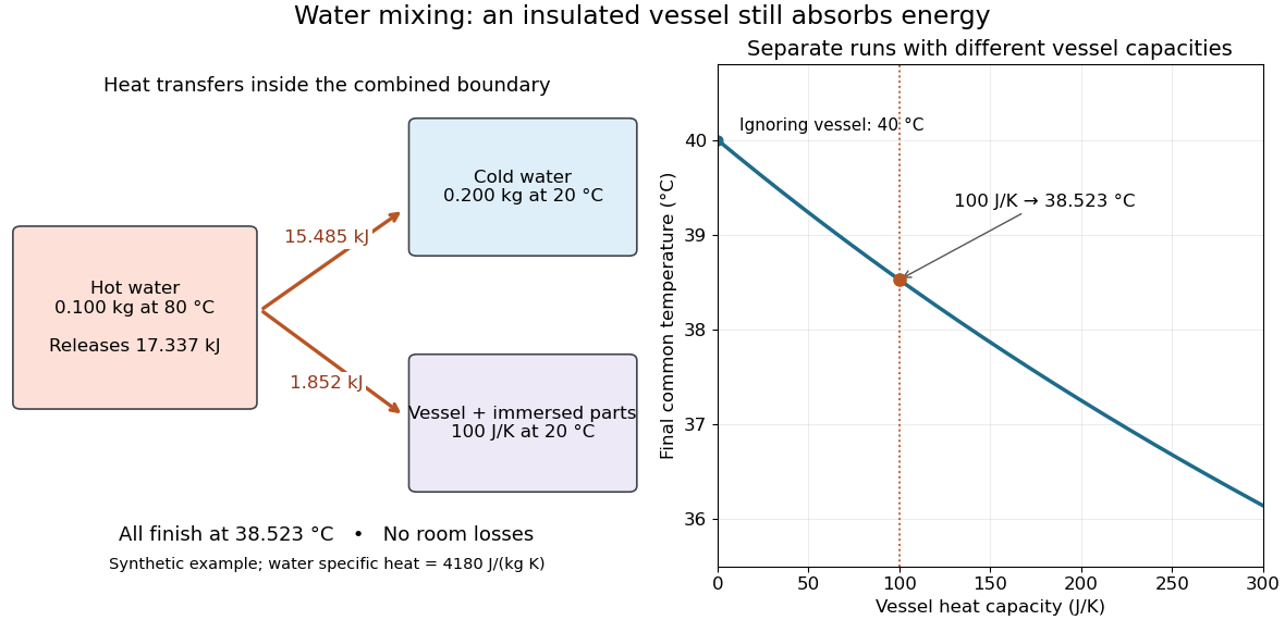
The vessel changes the mixing temperature by sharing the heat transfer
. Original computed no-loss water example. Left: transfers sum to the hot portion's released heat. Right: increasing the initially cold vessel's heat capacity lowers the common final temperature; the marked point uses . Each vessel setting is a separate modeled experiment. Details.For an unknown-sample example using the same cold water and vessel, stipulate , and . With no loss, . Inverting the full balance returns ; ignoring vessel storage returns about . With a positive outward loss, ignoring that loss also biases the inferred downward under these hot-sample conditions. A small water temperature rise makes sensor offsets and loss estimates relatively influential; propagation of uncertainty must include the measured temperatures, masses and calibrated vessel term.
A calibration is a closed real differential form whose comass is at most one. Restricting it to any oriented unit tangent plane therefore gives at most that plane's volume. A calibrated submanifold attains equality everywhere, and calibration implies volume minimization among homologous competitors.
An oriented submanifold is calibrated by a calibration when its tangent planes attain the comass bound at every point. Closedness then compares its volume with homologous competitors by Stokes theorem.
A generalized calibration bounds the full energy of a supersymmetric brane, including its potential or gauge couplings. For a membrane, compatible spinor bilinears obey . In a stationary gauge , Cartan's magic formula proves . The closed charge form then supplies the energy bound. This extends ordinary calibration from volume alone to charged branes, as developed in Topological charges for branes in M-theory.
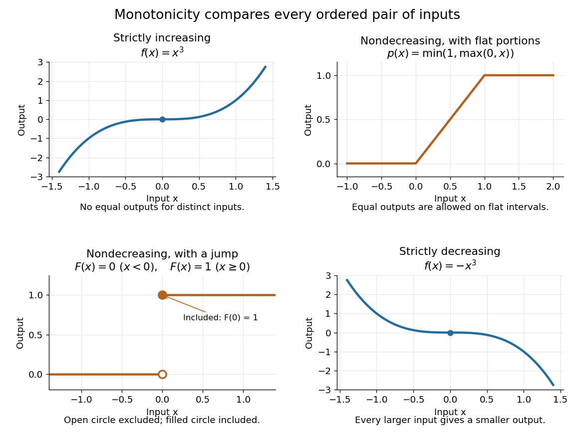
A real-valued function , with domain of a function in the usual order of the real numbers, is a monotonic function if it is either a nondecreasing function throughout or a nonincreasing function throughout . The same direction must work for every pair in . Being a strictly increasing function on one part and a strictly decreasing function on another does not make the whole function monotone: for example, on the real line changes direction at zero. A constant function is both a nondecreasing function and a nonincreasing function.
The word "increasing" is ambiguous across textbooks: some allow equal outputs and some require unequal outputs. Use nondecreasing function for the weak inequality and strictly increasing function for the strict inequality; use nonincreasing function and strictly decreasing function in the other direction. Neither continuity nor differentiability is part of the definition of a monotonic function.
Strict monotonicity gives injectivity, so an equation has at most one solution and an inverse function exists on the image of a function. Weak monotonicity permits repeated outputs and jumps. In probability theory, a cumulative distribution function is a nondecreasing function; its quantile function uses a generalized inverse to handle those flat parts and jumps. Monotonicity alone does not guarantee continuity, even for a strictly increasing function.
Taylor's theorem expresses a sufficiently differentiable function as a finite Taylor polynomial plus a Taylor remainder. One convenient version assumes is times continuously differentiable on the segment between and . Thenfor some intermediate point , when . Thus a bound on that segment gives . The intermediate point usually need not be computed: bounding the derivative throughout the segment is enough. This is why local approximation can yield reliable numerical bounds. A finite Taylor polynomial does not require an infinite Taylor series to represent the function.
Historically, the Royal Society holds Brook Taylor's letter of 26 July 1712 to John Machin. Its catalogue connects his work on Kepler's second law with the expansion later published in the 1715 Methodus incrementorum directa et inversa. This is a documented route from an orbital calculation to a general approximation method, rather than a claim that every earlier use of such expansions began with Taylor. See Royal Society archive, letter MS/82/2.
The floor function and ceiling function turn a real number into directed integer bounds. They answer two different questions: which integer is the largest one that does not exceed , and which is the smallest one that is not less than ?Both outputs are integers. These are exact mathematical operations; they need not choose the closest integer, and they do not refer to roundoff error in floating-point arithmetic.
For example,The fractional part is . The negative example matters: discarding the digits after the decimal point would give , which is truncation toward zero, rather than the floor function's value . At an integer, the floor function and ceiling function agree and the fractional part vanishes.
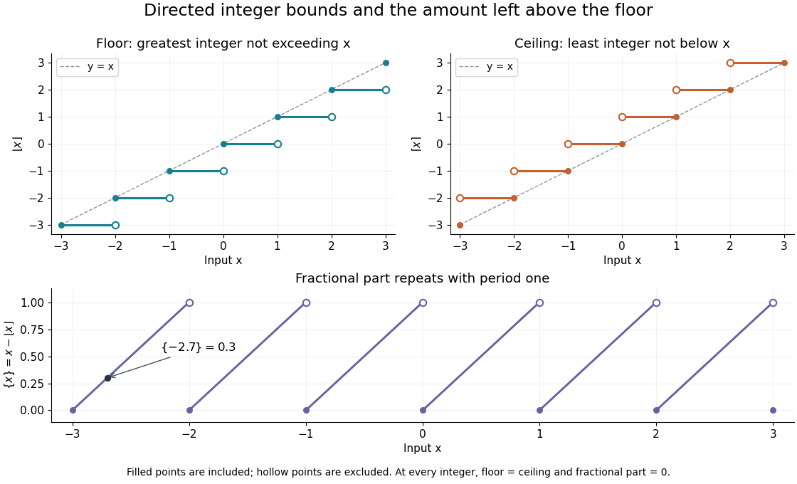


The usefulness is a bridge from continuous quantities to discrete decisions. An integer count in a closed interval uses both bounds. A ceiling count for fixed-size batches counts how many containers or pages are needed; a floor function counts how many complete groups fit. In Euclidean division, the same bounds specify the quotient, while the fractional part records the scaled remainder. A small amount of notation removes many cases that would otherwise have to be stated separately.
The reflection identityfollows by reflecting the ordered integers across zero: the largest one below becomes the smallest one above . For every integer , translation gives and . These formulas turn upper bounds into lower bounds and move examples between neighboring intervals.
For a historical example of the notation in use, Kenneth E. Iverson's 1962 conference paper A Programming Language lists the floor function, ceiling function and residue operation alongside the ordinary arithmetic operations. It states the two defining inequalities above, then extends operations component by component to vectors and matrices. This shows their role as tools for describing algorithms, rather than merely conventions for writing decimal numbers. [ref]
https://www.jsoftware.com/papers/AFIPS196205a.htm. Iverson, A Programming Language, AFIPS Spring Joint Computer Conference, May 1962, Basic Operations; transcription with typography changes documented at the end
Differential calculus studies derivatives: how a function changes near an input and how that local information describes its graph or evolution. Its tools include linear approximation, higher derivatives, and Taylor series; applications include finding velocity from position and studying optimization through critical points.
Metadata identifying which eligible backing cache block a valid cache slot currently holds. In the fully associative cache example, the cache tag is the full cache block number ; in the two-slot direct-mapped cache example, the slot supplies and the cache tag can store using the floor function.
An analytic semigroup is a strongly continuous semigroup whose bounded-operator-valued extension is holomorphic in a sector about the positive time axis. Its infinitesimal generator of a semigroup satisfies for and, on each bounded time interval, . This estimate gives instantaneous spatial smoothing but creates an integrable-singularity question in an inhomogeneous variation-of-constants formula.
A forecast horizon is the duration over which a prediction meets a specified error tolerance. If an initial uncertainty grows approximately as with positive Lyapunov exponent , then solving for when it reaches a tolerance gives the displayed estimate. Here is the natural logarithm and is measured per step of the discrete dynamical system; for a flow map, use the exponent per unit time instead. The estimate assumes the growth approximation remains valid up to the chosen tolerance and excludes additional model errors.
Reducing by a factor ten buys approximately more steps, rather than multiplying the forecast duration by ten. For typical logistic map orbits at , , so one extra decimal digit buys roughly steps in this approximation. Better measurements help, but their benefit is logarithmic. A forecast of a probability distribution or a stable long-term average asks a different question from predicting each individual state.
Let a finite group act on a finite set , with an orbit-invariant weight in a commutative ring. Double counting gives the division-free identityIndeed, each is counted times, and each orbit contributes copies of its common weight. If is invertible in , dividing gives the weighted average formula of Burnside's lemma. For formal monomial weights one can first count over the integers and then specialize into any commutative ring; this avoids dividing by zero in modular characteristic.
For a permutation group, is the number of length- cycles of . The cycle index records the average cycle structure. On coloring a finite underlying set, a coloring fixed by is constant on each cycle. Replacing by the power-sum symmetric polynomial therefore gives the pattern inventory by the weighted Burnside lemma.
A dilute bubbly thermal is a rising, entraining fluid volume whose gas bubbles provide part of its buoyancy. With negligible bubble slip and gas loss, Boyle's law gives gas volume proportional to , where . Spherical fluid entrainment with normal entrainment velocity gives . Bubble concentration follows by dividing the gas volume by the growing thermal volume. A diameter-based Froude number closure is .
In the Boussinesq approximation, a spherical buoyant thermal with conserved total buoyancy obeys and , with . A zero-volume, zero-impulse point source gives , , where . Hence and . The zero-time singularity represents an ideal source limit, not a finite initially regular sphere.
Suppose identical buoyant thermals deliver buoyancy at rate to a mixed lower layer of area before penetrating its interface. Neglect source volume and heat loss. Relative to the upper-layer density, let , , and , where . The lower-layer buoyancy budget gives . A cycle-averaged fluid entrainment closure , with , , yields the displayed law. Neutrality of the thermal at the interface requires . The closure must incorporate the encounter duty cycle; an isolated-event entrainment law needs an additional averaging prescription.
A buffered device block whose identity is retained for unfinished work. Reference counting can represent both client references and additional pins. Dropping a client reference does not release an outstanding journal pin; dropping a pin does not remove somebody else's reference. In the buffer cache state model, counts all such retained references, so prevents buffer cache eviction. This count keeps the structure alive; a mutex separately controls who can inspect or change its contents. Waiting callers also need lifetime protection.
A valid buffered device block with no outstanding write obligation to the backing location tracked by this cache. It can serve a cache hit. It becomes eligible for buffer cache eviction only when its retention and any pending input-output permit reuse. “Clean” does not assert that a device's volatile memory cache has been flushed to persistent storage.
There are unlisted articles, also show them or only show them.