Finite subgroup of a field multiplicative group is cyclic by  Codex 0 Created 2026-09-24 Updated 2026-10-06
Codex 0 Created 2026-09-24 Updated 2026-10-06Every finite subgroup of is cyclic. If its exponent is , all its elements are roots of , so its size is at most ; finite abelian group theory supplies an element of order , forcing equality.
Let be an IID sample of real-valued random variables with finite expected value and finite variance , where . Its sample mean satisfiesLinearity of expectation gives the first identity. The variance of a sum and vanishing cross covariances give ; scaling by scales the variance by . Pairwise independent random variables with the same expected value and variance suffice for these identities, even without full independence. Grinstead and Snell state the corresponding finite-variance independent-trials result.[ref]
The standard deviation of the sample mean is . Four times as many observations halve this scale; they do not divide it by four. In the fair Bernoulli distribution example, , so sample sizes and give standard deviations and , respectively. The common-coin averaging example shows why merely repeating observations with a common marginal law does not justify this calculation.
Chebyshev's inequality turns the variance identity into a probability bound: for ,This proves convergence in probability of the sample mean to in this finite-variance setting, a form of the weak law of large numbers. It is an upper bound, so values above one convey no improvement over the universal probability bound one. Cauchy sample mean stability lies outside these hypotheses.
For integrable random variables on the same probability space and fixed real numbers , linearity of expectation statesThe random variables can be dependent random variables. The formula follows by the linearity of integration; a finite linear combination of integrable random variables remains integrable. For example, if takes with probabilities , then and are dependent random variables, yet .
An especially useful application counts how many events occur. Put , an indicator random variable, and . Since , we get . There is no need to compute the whole probability distribution of , or to assume independence. For a uniform random permutation of objects, each object stays fixed with probability , so the fixed point count of a uniform random permutation has expected value one for every . [ref]
https://ocw.mit.edu/courses/6-042j-mathematics-for-computer-science-spring-2015/mit6_042js15_textbook.pdf. Lehman, Leighton and Meyer, Mathematics for Computer Science, §18.5: linearity and sums of indicators
.Linearity of expectation concerns addition and multiplication by fixed scalars. Products instead satisfy under the hypotheses of expectation of a product of independent random variables. For the example above, , whereas . Applying a nonlinear function before averaging can therefore change the answer substantially; use the law of the unconscious statistician to compute that average.
The tail-sum formula expresses an expected value as the area under a survival function. For every nonnegative random variable ,This Lebesgue integral and the expected value may both be ; a probability density function is unnecessary. For a random variable taking values in the nonnegative integers, the corresponding sum isThe events and coincide because takes integer values. Thus the strict sum starts at zero, while the inclusive sum starts at one.[ref]
Random: Probability, Mathematical Statistics, Stochastic Processes by Kyle Siegrist. Expected Value, §2 Additional Properties, Right Distribution Function: nonnegative tail integral and integer-valued tail sums
For an original example, let the probability mass function of beIts expected value computed directly is . The strict tail probabilities at thresholds are : their sum is again . There is no probability mass at two, yet the event still has probability . The survival function has heights on the successive intervals ; each interval has length one, so its integral is the same sum.
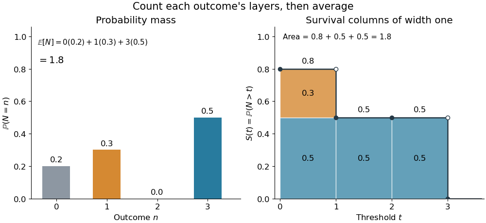
The same expected value from probability masses and survival columns
. The exact constructed probability mass function assigns to . The contribution appears in one survival column, while the contribution appears in three. Filled endpoints give the strict survival function at its jumps; open endpoints show the preceding height. The shaded area is . Details.
The indexing matters numerically. Starting the inclusive sum at zero adds , giving for this example. Starting the strict sum at one omits , giving . For a general nonnegative random variable, replacing with inside the integral is harmless: the difference is , nonzero at only a countable set of thresholds. For each positive integer , at most thresholds can have probability mass at least ; their countable union contains all thresholds with positive probability mass and has Lebesgue measure zero. This reasoning concerns an integral, not equality of the two survival function conventions at every point.
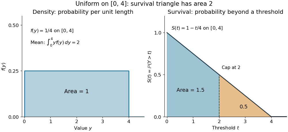
For a continuous original example, take the uniform distribution on the interval . Its survival function is for and zero for . The area is a triangle of base four and height one:Directly integrating against the probability density function gives the same expected value, . The integral of the probability density function alone is one; it is the survival function whose area is the expected value.

The proof counts layers of each outcome. For a realized value , the indicator function equals one over an interval of length , soTonelli theorem permits the interchange because the indicator function is nonnegative; no finite expected value is assumed. Similarly, an outcome contributes one indicator random variable for each of the events that occur:Again Tonelli theorem applies to the nonnegative sum, or equivalently the monotone convergence theorem applies to its partial sums. This exchanges counting layers within each outcome with averaging across outcomes. The existing integer-valued hypothesis in the tail-sum formula explains what changes when the values are not integers; the tail integral formula for moments weights the layers to obtain higher moments.
For an integrable random variable that can have either sign, apply the nonnegative formula separately to its positive part and negative part :Integrability makes both integrals finite. More generally the difference defines an extended expected value when at least one is finite; if both are infinite, subtraction does not define an expected value.[ref]
Random: Probability, Mathematical Statistics, Stochastic Processes by Kyle Siegrist. Expected Value, §2 Additional Properties, A General Definition: positive and negative parts and the condition on their expectations
Tail probabilities are often easier to measure or bound than a whole probability density function. For a device's survival time, the survival function records the probability of still operating at each threshold; its integral gives the mean operating time. A finite observation window naturally gives the expected value of a capped nonnegative random variable. For a mathematical bound, for all implies . The tail-sum formula turns control of a whole family of events into control of an average.
An indicator random variable is the indicator function of an event in a probability space: is one when occurs and zero otherwise. It has a Bernoulli distribution with parameter , so and . Even an event described without numbers becomes a numerical random variable in this way.
For a finite collection of events, their indicator random variables add up to the number that occur. Linearity of expectation therefore turns an average count into a sum of probabilities, without requiring independence. The fixed point count of a uniform random permutation provides an example where the indicators are dependent random variables.
The variance measures the mean squared distance of a random variable from its expected value. For a real square-integrable random variable ,The square prevents positive and negative deviations from cancelling. It also gives the variance squared units: if measures a length in metres, its variance has units of square metres. Its nonnegative square root is the standard deviation, which has the same units as .
For example, let take , and with equal probabilities. Its expected value is zero, but its variance is , and its standard deviation is . The constant random variable zero has the same expected value and zero variance: a mean alone does not describe the spread. The variance is zero exactly when almost surely.
The variance is useful because squared deviations interact neatly with linear combinations. The covariance supplies the cross terms when combining different random variables, and a covariance matrix organizes those terms for many variables. The characterization of variance as the minimum mean squared error of a constant also explains why the expected value is the best constant prediction under squared error.
For transmission through scale heights, a useful estimate isSmall host stars, low gravity, high temperature, and low mean molecular mass make atmospheric features larger.
Atmospheric escape removes gas from a planet through thermal motion, hydrodynamic outflow, photochemistry, and interactions with stellar radiation and plasma.
An exoplanet emission spectrum is the wavelength-dependent thermal radiation emerging from the planet. Vertical temperature gradients turn opacity differences into absorption or emission features.
An exoplanet transmission spectrum measures the wavelength-dependent area blocked as starlight passes tangentially through the atmosphere during transit.
An irradiated planetary atmosphere receives stellar energy from above while internal heat emerges from below. Their competition creates radiative, convective, and sometimes thermally inverted regions.
For oscillators of frequencies and , the perturbationpreserves . On the energy- basis , it is the matrixso the symmetric and antisymmetric combinations are exact eigenstates with shifts .
Let be a finite undirected multigraph, allowing self-loops and distinct parallel edges, with . Thenwhere is the edge support of a graph, and vertex degrees count each self-loop twice. There is no lower bound of three on the number of vertices. If , the zero-length convention gives an Euler circuit exactly when .[ref]
The two requirements are independent: two separate vertices, each carrying a self-loop, have even vertex degrees but disconnected edge support of a graph, so no Euler circuit can cover both edges.
Necessity follows because a single trail cannot cover edges in different connected components of a graph, while a closed trail pairs all arriving and departing incidences, including those at its starting vertex. For sufficiency, extend a trail using unused edges until no extension is possible. Even vertex degree parity prevents it from stopping anywhere except its starting vertex: a different stopping vertex would have an odd number of used incidences and hence at least one unused incidence. The result is a closed trail.
If unused edges remain, connectivity of the edge support of a graph supplies a vertex on the current closed trail with an unused incident edge. Removing a closed trail leaves even unused vertex degrees, so the same argument constructs another closed trail from that vertex. Splice it into the existing record. The two trails use disjoint edge identities, so the splice repeats no edge. Each splice uses more edges; finiteness ensures termination with an Euler circuit. This is the constructive idea of Hierholzer's algorithm.
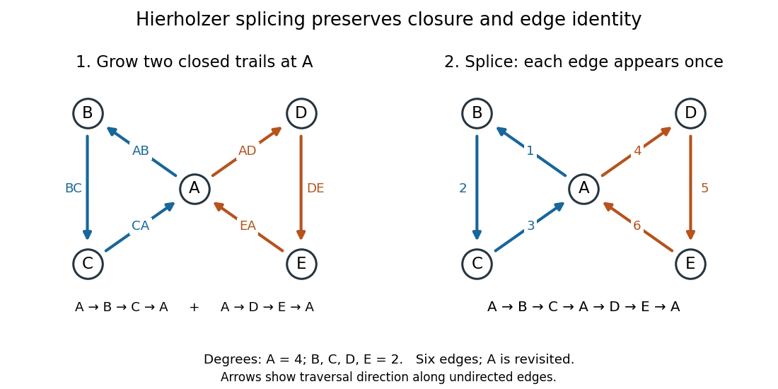
Hierholzer's algorithm inserts one closed trail into another at their shared vertex, using each of six edges exactly once
. Details. 
In the drawing, arrows indicate the chosen traversal direction along undirected edges. The first closed trail uses and the second uses . Insert the second at the final occurrence of in , giving . A reader can check consecutive endpoints, closure, and the six distinct edges directly. With multigraphs, perform the same check on edge identities, since endpoint pairs alone cannot distinguish parallel edges.
The Gibbs-Duhem equation constrains changes of the intensive quantities describing one uniform thermodynamic phase. For a mixture with independently specified component amounts, its molar form isHere is entropy, is volume, is temperature, is pressure, is the amount of substance of component , and is its molar chemical potential. This assumes a simple compressible system whose bulk internal energy is an extensive quantity; additional work coordinates require additional terms.[ref]
Thermodynamics and Chemistry by Howard DeVoe. Howard DeVoe, Thermodynamics and Chemistry, second edition, version 10, §9.2.8, printed p. 240, equations 9.2.42–9.2.44
The proof exposes the source of the constraint. For internal energy , replication of the whole thermodynamic phase by a factor gives . The Euler theorem for homogeneous functions and the fundamental differential of internal energy therefore giveTaking the differential of the first equation produces all the terms in the second, plus . Subtraction proves the Gibbs-Duhem equation. Thus the constraint comes from two descriptions of the same state function, rather than an assumed microscopic interaction model.
At fixed temperature and pressure, divide by and introduce the mole fractions :The chemical potentials cannot be varied independently. In a two-component mixture, put and . Within a smooth single-thermodynamic phase region with ,One chemical potential fixes the other's change, but determining its absolute value still requires a reference value. This does not say : equality at phase coexistence concerns the same chemical species in different thermodynamic phases. Nor does the constraint say whenever temperature and pressure are fixed; changing composition still contributes to the Gibbs free energy.
There are unlisted articles, also show them or only show them.