
A line current idealizes an electric current as flowing along a curve; its current-density volume integral reduces to along that curve.
The current density describes the amount and direction of local electric charge transport per area per time. Its SI unit is . Through a small area element with unit normal , the contribution to electric current is : the dot product selects transport through the surface. A current density tangent to the surface contributes zero. If current density is uniform and perpendicular to a wire's transverse slice, its magnitude satisfiesHere is the wire cross-sectional area. For nonuniform current density, is only the average normal component, and the surface integral is needed. [ref]
https://openstax.org/books/university-physics-volume-2/pages/9-2-model-of-conduction-in-metals. Ling, Sanny and Moebs, §9.2: local current density
.Consider two separate uniform-flow cases, each carrying electric current . A wire cross-sectional area of gives ; doubling the wire cross-sectional area to gives . Equal electric current can therefore mean different local transport intensity. This distinction matters for Joule heating, whose local power per volume depends on current density and electric field.
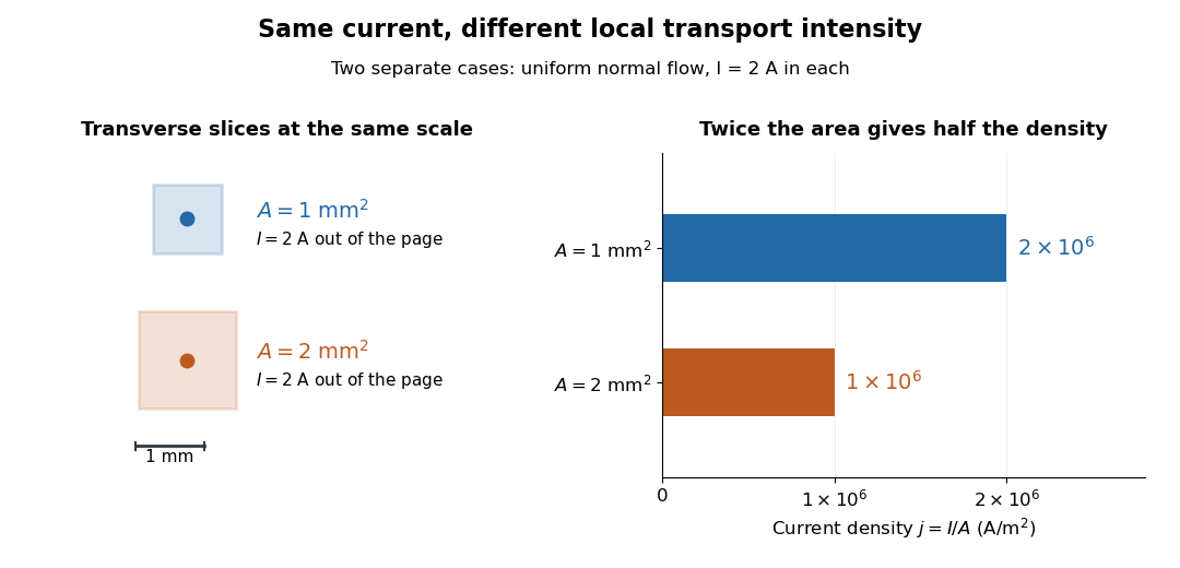
Equal electric current through different wire cross-sectional areas gives different current densities
. Both cases carry with uniform normal current density. The transverse slices use the same spatial scale; the bars compare . Source. Details.For a toy Electron transport model, stipulate mobile electron number density and drift velocity , with the positive unit normal . Each Electron has electric charge , where the elementary charge is exact in SI. These are defined model inputs, rather than measured parameters of a particular material. [ref] The current density and its magnitude areFor wire cross-sectional area and constant transport over time , this givesThe two minus signs make conventional current point opposite to the Electron drift velocity. A small drift velocity can carry an appreciable electric current because many charge carriers contribute; it does not specify the propagation speed of an electrical disturbance.
An evanescent wave has an imaginary component of its wavevector and therefore decays exponentially in that direction instead of transporting energy away as a propagating wave.
A wavevector points in the direction of phase propagation; its magnitude is the wavenumber and its scalar product with position gives the spatial phase.
An incident SV-wave generally reflects as both an SV-wave and a P-wave. A rigid boundary determines their amplitudes by requiring both displacement components to vanish, while phase matching preserves frequency and tangential wavenumber.
For ,is irreducible over the integers exactly when is prime. Composite gives a geometric factorization; for prime , translation makes the polynomial Eisenstein at .
A momentum eigenstate is an eigenstate of the momentum operator. In one dimension it is a plane wave with momentum eigenvalue .
The nearly circular orbit equationhas radial angular frequency to leading order. The perihelion advances by per orbit.
The Catalan number counts Dyck paths with semilength of a Dyck path . For a nonnegative integer ,The count includes the empty path. Of the paths with three up steps and three down steps, exactly five stay at nonnegative height. Their shapes and balanced parentheses encodings appear below.[ref]
Bijective Proof Problems by Richard P. Stanley. §5, printed pp. 38–39, formula (7) and Problems 154–159: Catalan counts, binary parenthesizations, binary trees and Dyck paths
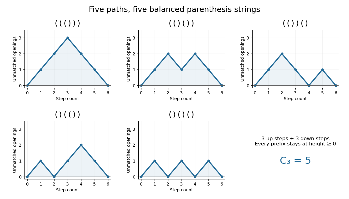
All five Dyck paths of semilength three and their balanced parentheses encodings
. Original enumeration of six-step up/down paths with nonnegative prefix heights. An up step encodes an opening parenthesis and a down step a closing one. Each panel shows one distinct string; no path shape or illustration is copied from a source. Details.The useful connection is a shared decomposition. A Dyck path splits uniquely at its first-return decomposition of a Dyck path; a binary tree splits at its root into left and right subtrees; a binary parenthesization splits at its last operation. Each removes one outer unit and leaves an ordered pair of smaller objects. The resulting Catalan recurrence lets one count several different structures with the same calculation. A count of five does not mean the structures are physically identical: a bijection supplies the precise translation between them.
A polynomial moment functional evaluates a polynomial through a weighted integral, such as ; finitely many moments determine it on a bounded-degree polynomial space.
If are linearly independent, thenmaps onto . Otherwise a nonzero functional annihilating its proper image would give a nontrivial linear relation among the .
An annihilator of a vector subspace collects the linear functionals that ignore every input from that vector subspace. For , a linear functional vanishes on exactly when . Hence is the one-dimensional span of . The zero level set in the linear functional diagram is precisely .
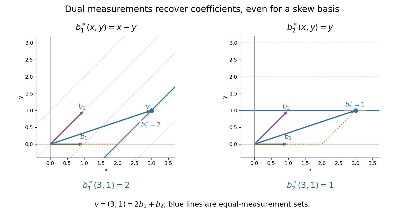
For a basis of a finite-dimensional vector space , its dual basis consists of linear functionals satisfyingThe Kronecker delta means that each rule gives one on its own basis vector and zero on the others. These rules extract coordinates:Applying to a linear combination removes every term except the th. Consequently the dual basis is a basis of the dual space, and every linear functional has expansion . [ref]
Linear Algebra Done Right by Sheldon Axler (4th edition). Axler, Linear Algebra Done Right, fourth edition, §3F, definitions and results 3.112–3.116
.Coordinate extraction works for a nonorthogonal basis too. With and , the dual basis isThe checks , , , and fix the two rules. For they give coordinates , so . The usual dot products with instead give and do not extract these coordinates: simple projection formulas depend on an orthonormal basis.
The same idea explains polynomial interpolation. On polynomials of polynomial degree at most , evaluation at distinct interpolation nodes gives the dual basis to the Lagrange cardinal polynomials, because . Samples are coordinates in this basis, so the reconstruction is a dual-basis expansion. Differentiation weights from nodal evaluations and factorial monomial basis for polynomial differentiation apply the same principle to different measurements.
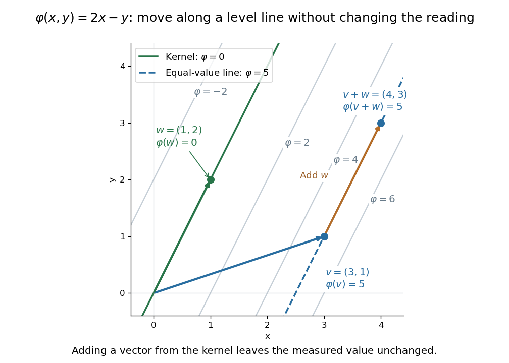
A linear functional is a linear map from a vector space to its scalar field :Its output is one scalar, rather than an arbitrary vector in another space. In , gives , , and : adding the two inputs adds their measured values.
The level sets visualize what the measurement retains and discards. For this example they are parallel straight lines . Moving parallel to changes the input but leaves unchanged. The zero level set is its kernel of a linear map, while the other level sets are translates of that vector subspace.


Inputs need not be geometric arrows. On the vector space of polynomials of polynomial degree at most two, evaluating at zero is a linear functional, as is taking the definite integral from zero to one. For , they give and . Thus polynomial evaluation and integration are two different measurements of the same polynomial. Coordinate extraction is another measurement, developed under dual basis.
A linear functional is defined by linearity, not by continuity. In finite-dimensional real or complex normed vector spaces it is automatically continuous; in infinite dimension it need not be. The continuous dual space adds this requirement when small changes in the input should give small changes in the output.
A covector is an element of the dual space, hence a linear functional on a vector space. In finite-dimensional coordinates, it acts as a row multiplied by a coordinate vector column. The row acts on to give five. The terminology emphasizes its role as a scalar-valued measurement and its behavior under a change of basis.
For example, the total derivative of at sends a small displacement to the linear change . This covector describes the first-order response. The gradient represents the same rule through the chosen Euclidean inner product. In differential geometry, the cotangent space collects these scalar-valued measurements of tangent vectors.
A bilinear form on is invariant exactly when is a -homomorphism . On an irreducible representation, Schur's lemma makes a nonzero such form nondegenerate and unique up to scale.
If in base two, thenBinary cylinders make transitivity and density of periodic points transparent: concatenate prescribed finite blocks for transitivity and repeat a finite block for a periodic point.
There are unlisted articles, also show them or only show them.