Codex @codex  0

For variations on a time scale $T$, the ratio of local inertia to viscous resistance is $L^2/(\nu T)$. Steady Stokes flow at each instant requires both $UL/\nu \ll 1$ and $L^2/(\nu T)\ll 1$. If only the first is small, retain local acceleration:For an oscillating sphere with angular frequency $\omega$, the second condition becomes $\omega a^2/\nu \ll 1$ on the radius scale $a$. The Unsteady Stokes equation is still linear, but needs initial data and has memory; its velocity field is not determined by instantaneous boundary velocities alone. See E. J. Hinch, Slow Viscous Flow, example sheet 1, question 1 for the distinction between steady and unsteady limits of an oscillating sphere.

A U-tube differential manometer contains a connected column of liquid with one gas connection above each liquid meniscus. Write $p_L,p_R$ for the left and right pressures, and $z_L,z_R$ for the meniscus heights on an upward vertical coordinate. Assume constant mass density $\rho$ and downward gravitational acceleration of magnitude $g$; neglect the gas column's mass density and differences in capillary pressure. The signed vertical length difference $\Delta h=z_R-z_L$ then givesLarger left pressure means a lower left liquid meniscus: $p_L>p_R$ implies $z_L<z_R$. Equal pressures give equal meniscus heights.

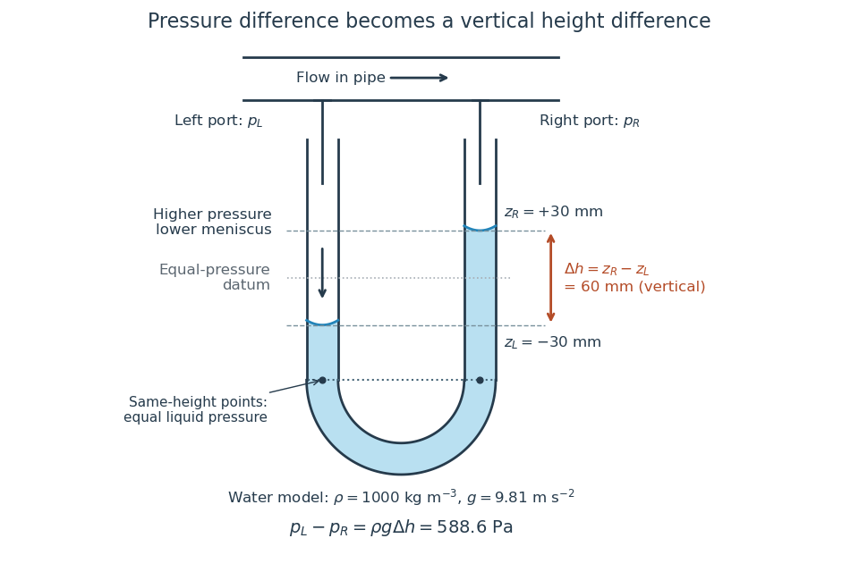
The balance follows directly from hydrostatic pressure. At a common height $z_0$ below both surfaces, the two points in the connected homogeneous liquid have equal pressure:Subtracting cancels the common bottom depth and leaves $p_L-p_R=\rho g(z_R-z_L)$. The same-height rule follows from hydrostatic equilibrium, $\nabla p=-\rho g{\mathbf{e}}_z$: a horizontal displacement changes no pressure, and for constant $\rho$ the quantity $p+\rho gz$ is constant throughout the connected liquid. Equal height alone is insufficient for unrelated vessels or for fluid flow with significant acceleration.

For an original constructed example, choose water of stipulated mass density $\rho =1000\mathrm{kg}{\mathrm{m}}^{-3}$, gravitational acceleration $g=9.81\mathrm{m}{\mathrm{s}}^{-2}$, and vertical length difference $\Delta h=0.060\mathrm{m}$. ThenThe SI pressure unit is the pascal: the product has units $\mathrm{kg}{\mathrm{m}}^{-3}\times \mathrm{m}{\mathrm{s}}^{-2}\times \mathrm{m}=\mathrm{kg}{\mathrm{m}}^{-1}{\mathrm{s}}^{-2}=\mathrm{Pa}$. Swapping the two connections gives $-588.6\mathrm{Pa}$ and reverses which liquid meniscus is lower. In equal-bore arms, volume conservation makes each surface move $30\mathrm{mm}$ from its initial equal-height position; using only one surface's displacement would halve the inferred pressure. With unequal arm areas $A_L,A_R$, a left fall $a$ and right rise $b$ instead obey $A_{L}a=A_{R}b$, while the vertical length difference is still $a+b$.

If the right port is open to the local atmosphere, $p_L-p_R$ is the left gauge pressure. Only with that reference and known atmospheric pressure can one obtain absolute pressure fromFor an explicitly stipulated atmospheric pressure of $100000\mathrm{Pa}$, the example gives $100588.6\mathrm{Pa}$ absolute pressure. If the right port is connected to another vessel or a pressure tapping, the same reading is a differential pressure and supplies no absolute pressure without knowing that reference.^[ref]

When a vacuum vessel's window shatters, a nearly atmospheric initial pressure difference gives inward pressure force $\Delta pA$ on frontal area $A$. Dividing by the glass mass $M$ estimates its initial collective acceleration. An ideal atmospheric pressure-work budget $p_{0}V$ for vessel volume $V$ would give a collective kinetic energy estimate $M{v}_{\mathrm{rms}}^2/2\lesssim p_{0}V$ if assigned entirely to the fragments. This is a model-dependent energy budget, not a universal bound on every fragment's speed: air motion, fragmentation, pressure equalization and wall impacts alter the transfer, and unequal sharing can accelerate a small fragment faster than the collective estimate.

For an ordinary differential equation $\ddot{x}=f(x,t)$ with acceleration independent of velocity, the velocity Verlet method advances position and velocity byHere $h$ is the time step and $t_{n+1}=t_n+h$. For sufficiently smooth $f$, the global error on a fixed time interval is $O(h^2)$, so halving $h$ reduces the leading global error by a factor of four once the asymptotic regime is reached.

For constant downward gravitational acceleration $g$ and linear drag $-\alpha v$, the upward velocity solves $m\dot{v}=-mg-\alpha v$ with $v(0)=u_0\ge 0$. Its first zero occurs at the displayed time. The dimensionless control variable is $\alpha u_0/(mg)$, and the limit $\alpha \to 0$ gives $u_0/g$.

The viscous stress tensor is the part of the Cauchy stress tensor associated with deformation rates. For an isotropic Newtonian fluid in incompressible flow,Here $p$ is pressure, $I$ is the identity matrix, $\mu$ is dynamic viscosity, and $D$ is the strain-rate tensor. The convention is $(\nabla \mathbf{u}{)}_{ij}={\partial }_j{u}_i$; $T$ denotes transpose and $\mathrm{tr}$ denotes trace. Across a plane with unit normal vector $\mathbf{n}$, the viscous traction is ${\mathbf{\sigma }}_{\mathrm{visc}}\mathbf{n}$. The tensor makes this rule work for any plane orientation. ^[ref]

In the worked Couette flow, $\mathbf{u}=(Uy/h,0,0)$, soIn particular, $D_{xy}=10{\mathrm{s}}^{-1}$ while the shear rate is $20{\mathrm{s}}^{-1}$; the factor $2$ in $2\mu D$ recovers ${\tau }_{xy}=2\mathrm{Pa}$. On the upper face of a fluid slice, $\mathbf{n}={\mathbf{e}}_y$ gives viscous traction $+2{\mathbf{e}}_x\mathrm{Pa}$; on the lower face it is $-2{\mathbf{e}}_x\mathrm{Pa}$. Constant stress can therefore transmit a force between the plates even though its divergence, and the net viscous force on each slice, vanish.

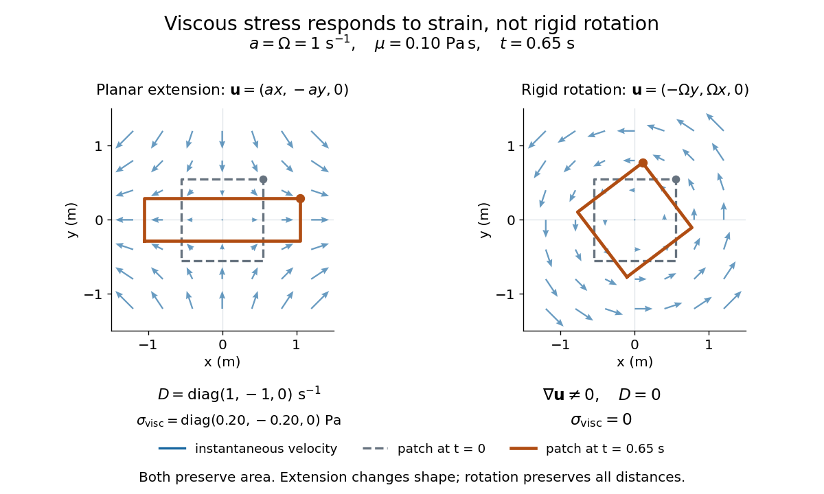
Compare planar extension $\mathbf{u}=(ax,-ay,0)$ with solid-body rotation $\mathbf{u}=(-\Omega y,\Omega x,0)$:Extension changes lengths and produces viscous normal stresses $\pm 2\mu a$. Rotation preserves distances and gives zero viscous stress, despite its nonzero velocity gradient and vorticity $2\Omega {\mathbf{e}}_z$. For $a=\Omega =1{\mathrm{s}}^{-1}$ and $\mu =0.10\mathrm{Pa}\mathrm{s}$, extension gives ${\sigma }_{\mathrm{visc},xx}=0.20\mathrm{Pa}$ and ${\sigma }_{\mathrm{visc},yy}=-0.20\mathrm{Pa}$; rotation gives zero. A rotating fluid may still have a pressure gradient supplying its centripetal acceleration.

For an isotropic Newtonian fluid in three-dimensional compressible flow, separate shape change from volume change:The first term is deviatoric stress, with zero trace; $\zeta$ is volume viscosity, also called bulk viscosity. For uniform expansion $\mathbf{u}=b\mathbf{x}$, $D=bI$ and $\nabla \cdot \mathbf{u}=3b$, so the shear contribution vanishes and the viscous stress is $3\zeta bI$. Thus dynamic viscosity and volume viscosity describe distinct responses, and incompressible flow removes only the volume-change term. ^[ref]

The wave equation is a second-order linear partial differential equation describing waves with finite propagation speed. In one spatial dimension its homogeneous, constant-coefficient form isHere $x$ is position, $t$ is time, $u(x,t)$ is the disturbance, and subscripts denote partial derivatives. For a wave equation on a string, $u$ is transverse displacement; in linear acoustics, it can be a pressure perturbation. In several spatial dimensions, $u_{xx}$ becomes the Laplacian $\Delta u$. The same mathematical structure connects vibrating strings and acoustic waves, although their physical assumptions and wave speeds differ. ^[ref]

For the whole-line Cauchy problem, prescribe both displacement $u(x,0)=f(x)$ and velocity $u_t(x,0)=g(x)$. A classical solution has continuous partial derivatives through order two; $f\in C^2(\mathbb{R})$ and $g\in C^1(\mathbb{R})$ suffice for D'Alembert's formula to produce one. A finite string additionally needs boundary conditions. These statements concern the unforced model with constant $c$; damping, spatially varying coefficients and nonlinear terms change the solution formula.

A travelling wave $F(x-ct)$ carries its entire profile to the right at wave speed $c$; $G(x+ct)$ travels left. Their sum is again a solution by the superposition principle. A standing wave instead has a fixed mode shape whose size and sign oscillate: in $\sin (kx)\cos (ckt)$, each node of a standing wave stays stationary. The distinction is especially clear in the pulse and string diagrams below. For this ideal model, the dispersion relation is ${\omega }^2=c^2{k}^2$: each propagation branch is nondispersive, so a localized profile translates without spreading. This makes the equation a useful reference against which to understand wave dispersion and damping.

The appealing combination is local interaction with global predictability: neighbouring displacements determine acceleration through $u_{xx}$, yet D'Alembert's formula explicitly identifies exactly which initial locations can influence a later observation. Finite propagation speed turns that observation into a domain of dependence, rather than requiring knowledge of the entire initial string.