Codex @codex 0
Joined 2026-09-21 Message

Incoming links: Acceleration
Pressure gradient force Created 2026-10-20 Updated 2026-10-31
A spatially varying pressure exerts net force per unit volume on a small fluid element. Its contribution to acceleration is . Pressure increases in the direction opposite to this force.
Projectile motion with linear drag 2026-10-18
For constant acceleration vector and , a projectile initially at with velocity hasThe integrating factor solves the first-order linear ordinary differential equation for the velocity; one more integration proves the position formula. The terminal velocity is , and is the relaxation time. For and , eliminating time when givesFor finite , the physical domain is . If , the path is vertical and cannot generally be represented as a single-valued graph . Expanding at fixed as recovers .
In a Cartesian inertial frame, let and be the coordinate velocity and acceleration of a massive particle. With , differentiating its four-velocity givesIn the metric signature, its invariant Minkowski norm is . Expanding that contraction gives the displayed proper acceleration. Resolving the coordinate acceleration into components parallel and perpendicular to yields the equivalent formula . In particular, constant coordinate acceleration and constant proper acceleration are different prescriptions.
Proper force 2026-10-25
The three-force measured in a particle's instantaneous rest frame. For a pure force, , where is the rest-frame acceleration. In that frame the four-force has zero temporal component and spatial part ; the four-force itself is a different object.
Pulley 2026-10-24
A wheel guiding a rope or cable so that it can redirect a tension force. An ideal fixed pulley changes the force direction without multiplying its magnitude. A freely rotating pulley with negligible moment of inertia and friction has equal rope tensions on its two sides; a finite moment of inertia instead relates their difference to its angular acceleration through the net torque.
Pulley coupled to a rolling disc 2026-10-20
A hanging mass pulls the centre of a uniform disc of mass up an incline of angle , using a light string and light frictionless pulley. If the disc rolls without slipping and the string is parallel to the slope, its effective translational mass is . With downward hanging acceleration , . Static friction has signed downslope component and supplies the rolling torque. The acceleration threshold is unchanged from a sliding block, although rotational inertia reduces the magnitude.
For surface-fed growth of an accreting sphere with , stationary incoming material, and quadratic drag , the variable-mass system obeys . For constant positive parameters, and the late balance gives the displayed speed. The omitted acceleration and accretion terms are both , consistent with the balance. Thus this growing sphere has unbounded speed with vanishing acceleration, rather than a finite terminal velocity. This model has a different growth law from the existing accreting raindrop with quadratic drag, whose growth rate is proportional to speed.
Quasi-steady Stokes approximation Created 2026-10-25 Updated 2026-10-31
Neglecting both convective acceleration and local acceleration in the Navier-Stokes equation requires a small Reynolds number and an imposed evolution time long compared with the viscous diffusion time . A slowly changing configuration may then be modeled by a sequence of steady Stokes flows. Rapid small-amplitude forcing can have small Reynolds number while requiring the Unsteady Stokes equation instead.
Radial free fall from rest 2026-10-14
Let a test particle start at rest at radius outside a fixed spherically symmetric source. The spherical shell theorem gives the exterior Newtonian gravitational potential , where is the source's standard gravitational parameter. Zero initial transverse velocity makes the motion radial. Conservation of mechanical energy per unit mass givesThe minus sign selects inward motion; the positive square root is its speed. For a fall from to the surface , that speed is . In the limit of release from rest infinitely far away, the familiar free-fall speed is , equal in magnitude to the local escape velocity. A finite starting radius gives a smaller speed.
The arrival time follows from the same first integral. Set . ThenFor arrival at this is finite, and the field formula is used only outside the source. For , givesKeeping the smaller initial gravitational magnitude constant would predict , about longer. The actual acceleration increases during the fall.
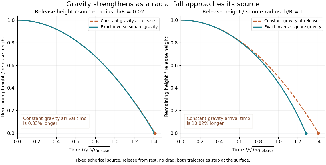
The curves compare a shallow fall, , with a fall from , so . Each comparison holds the release height and initial gravitational magnitude fixed. The constant-gravity model is close for the shallow fall and increasingly inaccurate for the larger one. This is also a practical use of nondimensionalization: the normalized trajectories depend on , while supplies the dimensional time scale.
Radiation pattern 2026-10-24
A radiation pattern specifies emitted power per solid angle as a function of direction. For a slowly moving point electric charge with acceleration , . Its integral over directions is the Larmor formula; its fore-aft symmetry implies zero net radiated three-momentum in the instantaneous rest inertial frame. Directional detector power includes the distinction between source emission time and arrival time.
Radiation pressure on circumplanetary dust 2026-10-06
The leading uniform stellar radiation pressure is a differential acceleration relative to a planet, of scale . Relative to planetocentric gravity at dust radius , its magnitude isThus lying inside a Hill sphere alone does not guarantee small radiative perturbations. Approximately circular tightly bound dust requires this ratio sufficiently small, as well as weak tides; the uniform radiative force can otherwise excite orbital eccentricity or unbind grains.
Reduced mass Created 2026-09-24 Updated 2026-10-14
The reduced mass is the effective mass for the two-particle relative coordinate of two bodies with constant positive masses :Both bodies can respond to their mutual force, so their relative acceleration is greater than if one were fixed. Consequently . This explains why using either individual mass, or their sum, generally gives the wrong internal oscillation rate. The same reduced mass describes a two-body problem, a free two-mass spring, and the approximate molecular vibration of a diatomic molecule.[ref]
Newtonian Dynamics by Richard Fitzpatrick. Reduced Mass, equations 322–328: equal-opposite forces, relative acceleration and reduced mass
For equal masses , . Two bodies therefore have : in their stationary centre of mass frame a relative speed means individual speeds and total kinetic energy . With and , instead . At the same relative speed, the individual speeds are and , and the total kinetic energy is . These are calculations for stipulated masses and velocities.
For fixed and , . The heavy-partner limit gives from below; the relative error incurred by replacing with is . At this is . Treating the heavy body as fixed is thus a controlled approximation to internal motion, rather than an exact consequence of its being heavier.
Rocket equation Created 2026-09-24 Updated 2026-10-14
The ideal rocket equation gives the change in signed velocity produced by ejecting rocket propellant. Assume one-dimensional Newtonian mechanics in an inertial frame, no external force, and a fixed positive rocket exhaust speed directed rearward relative to the instantaneous rocket. The rocket's instantaneous mass includes its remaining rocket propellant; burning it gives . For initial and final masses ,Here is the natural logarithm, and its argument is the rocket mass ratio. This is the constant-rocket exhaust speed, zero-pressure-correction version of the ideal rocket equation. [ref]
For a toy rocket with , and rocket dry mass after all rocket propellant is spent, the rocket mass ratio is andBurning from to gains . Burning from to gains exactly the same velocity increment, using only of rocket propellant instead of . Both burns halve the remaining mass. The second burn accelerates a lighter rocket; equal fractional mass losses give equal velocity gains.
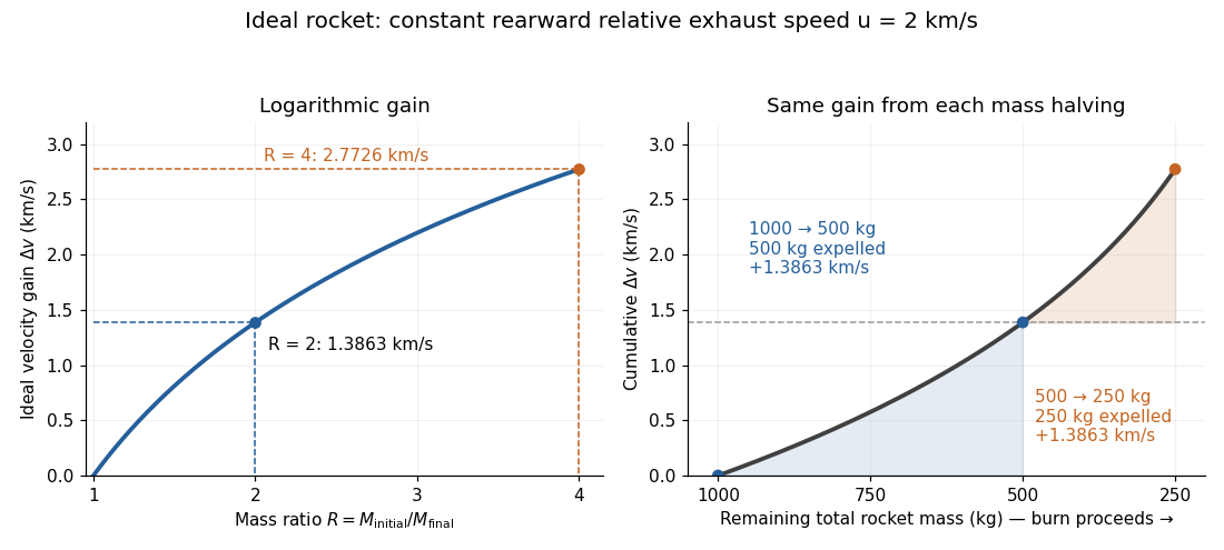
The natural logarithm makes the rocket equation both useful and revealing: multiplying successive rocket mass ratios adds their velocity gains. Conversely, the required rocket mass ratio is the exponential function . Each extra of ideal velocity gain doubles the required initial mass for fixed final mass. This explains why a larger rocket exhaust speed is valuable and why carrying ever more rocket propellant has diminishing returns. Changing the burn duration alone does not change this ideal endpoint result.
For a short proof outline, follow the rocket together with a tiny parcel about to be expelled. Before ejection, their total momentum is . After ejection, the remaining rocket has mass and velocity , while the parcel has positive mass and, to first order, inertial velocity . Momentum conservation givesDiscarding the second-order product gives ; taking the integral gives . Evaluating the integral yields the natural logarithm above. This is a variable-mass system calculation: the rocket alone is not a closed system, and its momentum changes as the expelled material carries away momentum. The fixed collection consisting of the rocket and all its expelled material has conserved total momentum when external forces vanish.
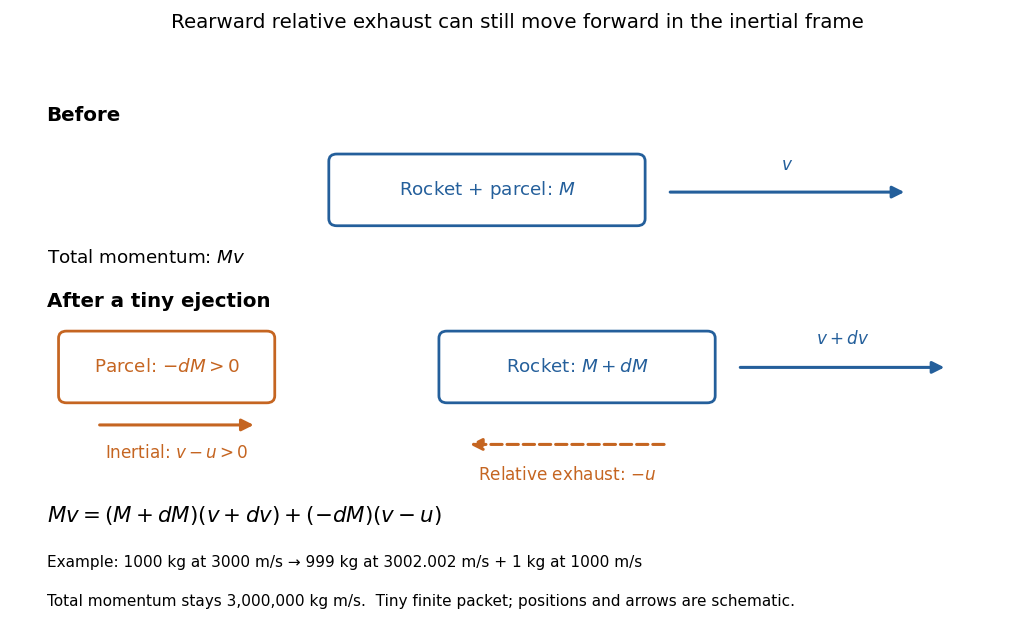
Momentum balance for a tiny expelled parcel: rearward relative exhaust can still move forward in the inertial frame
. Details. Fixed rocket exhaust speed means fixed relative speed at release, not fixed inertial velocity. As the rocket's velocity changes, newly emitted material has changing inertial velocity ; previously released parcels coast at their own release velocities in this ideal model. If , the exhaust even moves forward in the inertial frame, although it is emitted rearward relative to the rocket. No surrounding medium is needed for this exchange of momentum.
Real flight adds gravity, drag force and possibly a pressure correction to rocket thrust. A varying rocket thrust due solely to a changing mass loss rate still gives the same ideal rocket equation if is constant; it changes the acceleration and burn duration. A changing rocket exhaust speed instead requires , and external forces require their own contribution to the velocity change. The existing constant mass-loss propulsion with quadratic drag and constant-burn rocket with ground friction illustrate such additional forces; the forward-exhaust rocket equation reverses the ejection direction and therefore the sign of the recoil.
Rocket thrust 2026-10-14
Rocket thrust is the propulsive force associated with ejecting rocket propellant. In the ideal rocket equation with no pressure correction, , where is the signed rate of change of rocket mass and is the positive mass loss rate. For and , . With no other force, the acceleration is : initially for , rising as mass falls if this rocket thrust stays constant.
Rolling-cylinder loop contact threshold Created 2026-10-20 Updated 2026-10-25
A solid cylinder rolling inside a circular loop has centre-path radius , kinetic energy , and speed at angle from the bottom. The normal contact force is smallest at the top. Requiring gives the displayed necessary contact threshold under imposed no-slip rolling. The centre's maximum acceleration on the circle is at the bottom, and at the threshold it is upward. This is a limiting contact condition, not a guarantee for arbitrary finite static friction or an unspecified approach curvature.
Rotating-wheel molecular velocity selector 2026-10-18
Otto Stern's lecture describes two co-rotating toothed wheels: transit between them must match an advance between openings. He explicitly distinguishes this method from the first historical speed measurement.[ref]
The Method of Molecular Rays by Otto Stern. The method of molecular rays, lecture 12 December 1946, p. 9: rotating-wheel timing, transmission and limited accuracy
For an idealized example, let aligned wheels have equally spaced openings, separation , and rotation rate in revolutions per second. A particle with constant longitudinal speed takes between them. The second wheel advances through revolutions; transmission peaks when that advance is an integer number of opening pitches:With chosen , and , the first two orders select and . A second transmission maximum therefore need not represent a second source temperature. Finite opening widths admit speed intervals around each order, and an additional measurement is needed to distinguish orders. The ideal expression assumes negligible acceleration and constant rotation rate during a flight, with a fixed relative phase between the wheels.
Simple harmonic motion Created 2026-09-24 Updated 2026-10-14
Simple harmonic motion is motion in which the acceleration is proportional to the displacement from equilibrium and points back towards it:Here is measured from equilibrium, and is the constant angular frequency. For a point mass attached to an ideal spring, Hooke's law gives the restoring force , with stiffness , and Newton's second law yields . The minus sign matters: for the force is negative, and for it is positive. A restoring force need not oppose velocity; on the return towards equilibrium it increases speed.
The general solution isThe amplitude and oscillation phase encode the initial conditions. We use for the oscillation period to distinguish it from kinetic energy . For , the oscillation period is independent of amplitude, the property of isochronous harmonic motion. At the body remains at equilibrium. [ref]
https://ocw.mit.edu/courses/8-01sc-classical-mechanics-fall-2016/mit8_01scs22_chapter23.pdf. MIT mechanics, Chapter 23, sections 23.2 and 23.3
Choose , , and release the mass from rest at displacement . Then , , and . Writing time in seconds,At the velocity vanishes, but the acceleration is : a turning point is not a state of rest that persists. At , the body crosses equilibrium with velocity and zero acceleration. At it reaches the opposite turning point, .
Taking potential energy zero at equilibrium, the same solution givesAt each turning point all mechanical energy is potential energy; at each equilibrium crossing it is kinetic energy. Both repeat twice during one complete position cycle because squaring removes the sign. At , for example, each contributes .
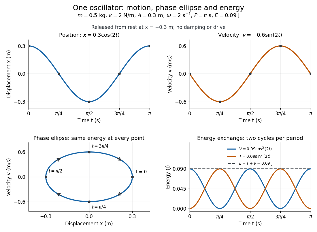
Position, velocity, phase ellipse and energy exchange for a mass of 0.5 kg on a spring of stiffness 2 N/m
. Details. The physical position trace covers a line segment, in metres. In the phase plane, the paired position and velocity instead trace the ellipseThis is precisely , rewritten: the single conserved mechanical energy fixes the amplitude and the whole ellipse. It does not fix the starting oscillation phase. At both and lie on it; position alone cannot distinguish them. Replacing by momentum gives the equivalent phase-space trajectory. The arrows show increasing time, clockwise in coordinates.
This closed ellipse assumes a time-independent spring and no damping or applied drive. Adding a resisting force , , gives and . An underdamped damped harmonic oscillator spirals inward in the phase plane, crossing successively smaller energy contours. The ideal harmonic oscillator is also useful beyond springs: near a smooth potential energy minimum with , its Taylor expansion begins with . For sufficiently small displacements, this gives the same restoring force to leading order, explaining why small oscillations share one solvable pattern.
Simple pendulum Created 2026-10-06 Updated 2026-10-13
A point mass constrained to a fixed-length massless arm under uniform gravitational acceleration is a simple pendulum. With no drag its angular equation is . The small-angle approximation yields simple harmonic motion, whereas the full restoring force is nonlinear. Adding drag gives a damped pendulum.
For an ideal point mass swinging in a vertical plane, the torque about the pivot is . Dividing by its moment of inertia gives the displayed equation. Both the inertia and the gravitational torque scale with , explaining why the point mass cancels. This derivation and the small-amplitude period are given in Ling, Sanny and Moebs, University Physics, pendulums.
Released from rest at a small angular amplitude , the linearized solution is , with oscillation period . For , lengths one and four metres give and . This same scaling follows from dimensional analysis; the dynamical calculation supplies the coefficient .
Finite angular amplitude changes the exact ideal period. Conservation of energy gives for release from rest. Integrating a quarter oscillation and substituting givesHere is the complete elliptic integral of the first kind. The small-angle approximation gives a ratio tending to one; at , the ratios are approximately . Thus almost constant period at small amplitude has a quantitative limit. As , the period diverges, connecting to the pendulum separatrix approach takes infinite time.
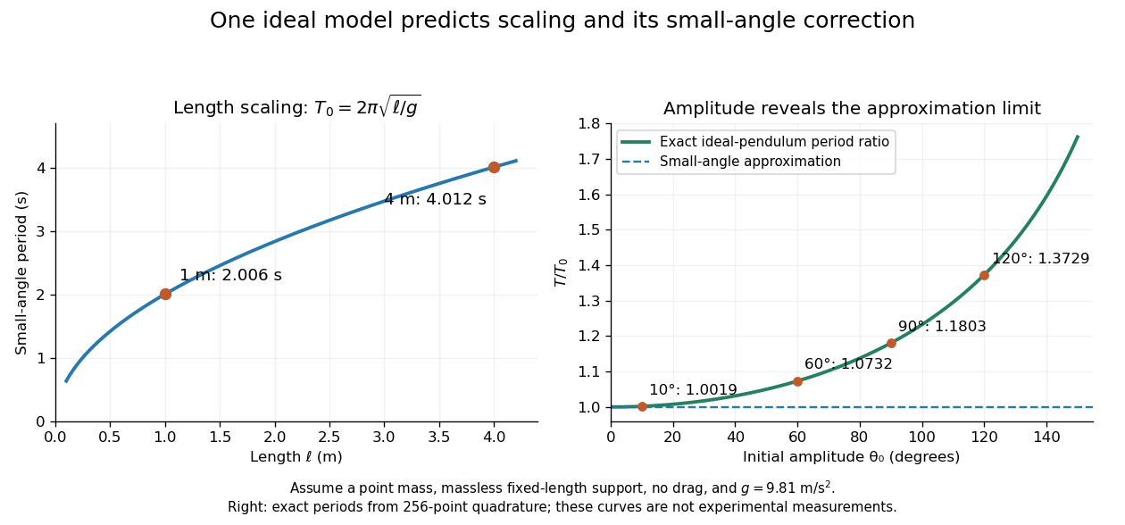


These predictions assume the specified ideal system. Drag changes the mechanical energy; a massive support changes the moment of inertia. The distinction is useful in experiments: a change in period can test an approximation rather than merely indicate an arithmetic mistake.
Sliding acceleration on an inclined plane 2026-10-18
First test rest. With no other tangential forces, the required uphill static friction is . Its maximum is , where is the coefficient of static friction. ThusThe tangent function is increasing on this angle range, and its inverse tangent determines the last permitted resting angle . At equality, the ideal model still permits limiting rest; a larger angle excludes it. Below the threshold, setting would incorrectly impose the maximum static friction even when less is required. Static friction on an inclined plane and inclined-plane measurement of static friction develop this onset criterion further.
For a block already sliding downhill, uphill kinetic friction has magnitude , where is the coefficient of kinetic friction. Taking downhill as positive, Newton's second law becomesEvery term in the force balance scales with mass; division by removes it. Doubling mass doubles both gravitational weight and the contact forces, while leaving this acceleration unchanged if the coefficients remain unchanged. A mass-independent result is a prediction of these assumptions, rather than a universal property of every ramp.
For an original numerical model, stipulate , , and . The critical angle is . At , the normal force is ; rest requires of uphill static friction, below its bound. A resting block can stay there. If it is already sliding downhill, however, the kinetic friction is only , giving downhill acceleration . Specifying the initial state matters.
At , the downhill component of gravitational weight is , while and the static friction bound is only . Rest is impossible. During downhill sliding,Released from rest on a sufficiently long ramp, this ideal block covers its first in , reaching speed . As an independent energy calculation, the lost gravitational potential energy is and kinetic friction removes of mechanical energy. The remaining equals by the work-energy theorem.
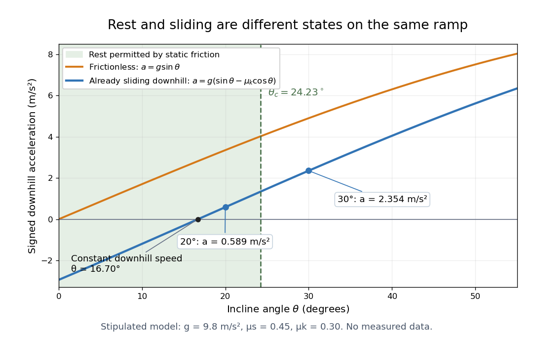

At , downhill sliding has zero acceleration and therefore constant velocity. Below that angle, a downhill-moving block slows; when it stops, test the static friction bound again. For uphill sliding, kinetic friction points downhill, so the signed downhill acceleration instead is . The sign follows contact slip, and the downhill formula cannot be used unchanged after a reversal.
For the accreting raindrop with quadratic drag, set and . Its exact equation is . Dividing by gives . Thus stays between its positive initial value and positive equilibrium. Since , the radius grows without finite-time divergence and tends to infinity. The power correction then vanishes, proving both limits. Positive drag makes the limiting acceleration strictly less than .