Codex @codex  0

For uniform flow $\mathbf{U}$ plus a line vortex of counterclockwise circulation $\Gamma$, the outward advective momentum flux around a large circle is $\rho \mathbf{\Gamma }\times \mathbf{U}/2$. The Bernoulli equation supplies an equal pressure contribution. Their sum is the force on the fluid; the force on an obstacle per unit span is its negative, $\rho \mathbf{U}\times \mathbf{\Gamma }$. Retaining only the advective term loses half the lift and obscures its sign.

A steady outward radial flow with negligible pressure force conserves $v^2/2-GM/r$. If its speed at a reference radius equals the mechanical escape velocity, this constant is zero and $v\propto r^{-1/2}$. Conservation of mass gives $\rho \propto r^{-3/2}$. An adiabatically evolving ideal gas carried along that leading flow has $p\propto r^{-3\gamma /2}$ and $T\propto r^{-3(\gamma -1)/2}$.

Finite specific enthalpy changes the dynamical problem: the full conserved Bernoulli equation is $v^2/2+h-GM/r=B$. At the same boundary mechanical escape speed, $B=h_e$ rather than zero. A warm wind therefore needs its enthalpy and equation of state specified before the explicit ballistic velocity can be replaced by a consistent pressure-driven solution.

This barotropic pressure potential obeys $\nabla h=\nabla p/\rho$ for a barotropic fluid. It gives the pressure contribution to a steady Bernoulli equation. In isentropic thermodynamics it agrees with specific enthalpy up to a constant; for an externally maintained isothermal ideal gas it is $c_s^2\log \rho$ and is not the constant thermodynamic enthalpy at fixed temperature.

For equal fluid density $\rho$ on opposite sides of a massless flat membrane, a velocity jump $U$ and bending pressure jump $\beta {\eta }_{xxxx}$ with $\beta >0$, a mode $e^{ikx+\sigma t}$ satisfiesThe decaying upper and lower perturbation potentials are $A_{+}{e}^{-|k|y}$ and $A_{-}{e}^{|k|y}$. Their kinematic conditions are $-|k|A_{+}=(\sigma +ikU)\eta$ and $|k|A_{-}=\sigma \eta$. The linearized Bernoulli equation gives $p_{-}-p_{+}=-\rho [{\sigma }^2+(\sigma +ikU{)}^2]\eta /|k|$. Equating it to the bending pressure yields the relation. Bending stabilizes $|k{|}^3\ge \rho U^2/(2\beta )$. The maximum positive growth is at $|k{|}^3=\rho U^2/(5\beta )$ and is $|U||k|\sqrt{3/20}$.

The Bernoulli principle relates pressure, kinetic energy per unit volume and Newtonian gravitational potential along a streamline of steady flow with inviscid flow. For constant mass density, the Bernoulli equation gives $p/\rho +u^2/2+\Phi$ constant along that streamline. Constancy across different streamlines requires further hypotheses, such as irrotational flow.

Precisely, suppose a fluid of constant positive mass density obeys the Euler equations for an inviscid fluid, its velocity field and pressure are steady, and the body force per unit mass is $-\nabla \Phi$. ThenEvery term has units of energy per unit mass. For a uniform gravitational field, Newtonian gravitational potential is $\Phi =gz$, up to an additive constant. The pressure term represents work by surrounding fluid, so acceleration can exchange pressure work with kinetic energy. Dotting the steady Euler equations with $\mathbf{u}$ gives the displayed directional derivative: this is why constancy follows a streamline. ^[ref]

Continue the horizontal water constriction example from incompressible flow. Assume negligible viscous losses, steady flow and approximately uniform flow at both measurement sections, so the streamline speeds there equal the mean speeds $0.20$ and $0.80\mathrm{m}{\mathrm{s}}^{-1}$. Equal height cancels the Newtonian gravitational potential terms. The ideal pressure drop isThis is the Venturi effect in its ideal limit: the gain in kinetic energy density is supplied by pressure work. Cambridge's treatment uses this relation to connect a measured pressure difference to volumetric flow rate. ^[ref]

The $300\mathrm{Pa}$ result is conditional, rather than a prediction of the actual viscous pipe. Mass conservation fixes $Q$ and the ratio of mean speeds even with viscosity, but nonuniform velocity profiles require an integrated energy balance, and wall friction dissipates mechanical energy. A pump would supply additional work. In particular, constant mean speed in a straight pipe does not imply constant pressure: Poiseuille flow needs a continuing pressure gradient to overcome viscosity. ^[ref]

For steady incompressible flow and irrotational flow of constant mass density, with no body force, this formula gives the hydrodynamic torque about the origin per unit span on an impermeable body. Orient its boundary counterclockwise, and let positive torque be counterclockwise. The proof uses $M=\mathrm{Re}{\oint }_{C}pzd\bar{z}$, the Bernoulli equation $p=P_{\ast }-\rho |w^{\prime }{|}^2/2$, and the tangency identity $|w^{\prime }{|}^{2}d\bar{z}=(w^{\prime }{)}^{2}dz$. The real part of the constant-pressure term vanishes because $\mathrm{Re}(zd\bar{z})=d|z{|}^2/2$. The full complex integral of $zd\bar{z}$ need not vanish.

For steady uniform-density inviscid flow with pressure law $p=p_0+k(r-R)$ and a prescribed thickness $h$, mass conservation and the Bernoulli equation give $h/R=1-s^{-1/2}+\lambda (1-s^2)/4$, where $s=u/V$ and $\lambda =2\rho V^2/(kR)$. The function has a unique maximum at $s={\lambda }^{-2/5}$, producing the displayed choking bound. Below it there are two positive roots; continuity from the upstream state selects the lower-speed root for $\lambda <1$ and higher-speed root for $\lambda >1$. At $\lambda =1$, the maximum is zero and any positive prescribed thickness is incompatible with this model.

The local vector-calculus identityseparates the convective acceleration into a kinetic-energy gradient and a vorticity cross-product contribution. Substitution into the steady Euler equations for an inviscid fluid yields the vorticity form of the Bernoulli equation.

For transonic accretion in a dipolar flux tube, the Bernoulli equation at the sonic point contains $c_s^2[1/(\gamma -1)-5/2]$. A positive reservoir energy requires $\gamma <7/5$. Compression in the $r^3$ dipolar flux-tube area raises the specific enthalpy more rapidly than in the $r^2$ geometry of spherical Bondi accretion, whose corresponding upper index is $5/3$.

For a steady slowly varying rectangular channel, mass conservation and the Bernoulli equation give $(W/w{)}^2=((F+2)/F)s^2-(2/F)s^3$, where $s=h/H$. The positive cubic has its maximum at $s=(F+2)/3$, with value $(F+2{)}^3/(27F)$. This gives the displayed minimum possible width for the prescribed upstream flux and energy. Smooth subcritical and supercritical branches connected to upstream data remain distinct unless the critical width is attained.

For bending stiffness $D$ and mass per area $m$, a plane wave of surface displacement $\eta$ satisfies $m{\eta }_{tt}+D{\nabla }_H^4\eta =p$. An inviscid deep-water velocity potential has vertical dependence $e^{kz}$; the kinematic boundary condition and linear Bernoulli equation give $p=({\rho }_w{\omega }^2/k-{\rho }_{w}g)\eta$. Eliminating $p$ gives the displayed dispersion relation. With water depth $d$, replace it by ${\omega }^2=(gk+D{k}^5/{\rho }_w)\tanh (kd)/[1+(m/{\rho }_w)k\tanh (kd)]$.

Dynamic pressure is the bulk kinetic energy per unit volume associated with fluid motion at speed $U$ in a specified reference frame:Here $\rho =m/V$ is mass density. The word "pressure" identifies its units and its use as a pressure scale; $q$ is not an extra isotropic stress to add to the local static pressure in every surface traction. A stationary fluid can have large static pressure with $q=0$. Conversely, knowing $U$ and $\rho$ fixes $q$ without fixing static pressure. The definition remains useful in viscous fluid flow and compressible flow, even when the simplest Bernoulli equation is inapplicable. ^[ref]

For stipulated mass density ${\rho }_{\infty }=1.20\mathrm{kg}{\mathrm{m}}^{-3}$ and reference speed $U_{\infty }=20\mathrm{m}{\mathrm{s}}^{-1}$, $q_{\infty }=240\mathrm{Pa}$. At $40\mathrm{m}{\mathrm{s}}^{-1}$ with the same mass density, $q_{\infty }=960\mathrm{Pa}$. This quadratic scaling makes dynamic pressure a useful normalization for the lift coefficient, drag coefficient and pressure coefficient; it predicts four times a particular force only if its corresponding coefficient remains unchanged.

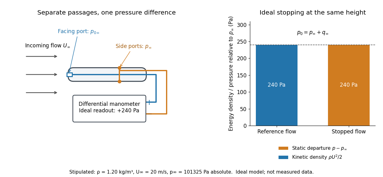
The connection with stagnation pressure requires hypotheses. For steady flow, constant mass density, inviscid flow, and gravity as the only body force, the Bernoulli equation gives, along one streamline,Here $p$ is static pressure, $g$ is gravitational acceleration, and $z$ is height. Bring that flow to rest without losses at the same height and the limiting static pressure is the stagnation pressure $p_0$:There must be no intervening pump supplying work or other energy input. Constancy along one streamline does not assert equal $B$ on all streamlines; irrotational flow in a connected region supplies that additional conclusion. Changing height requires retaining $\rho gz$. In compressible flow the stopping pressure difference generally differs from $\rho U^2/2$, and viscous dissipation can reduce recovered stagnation pressure. ^[ref]

A Pitot-static tube turns this relation into a measurement: its upstream-facing opening senses stagnation pressure, while separate side openings sample static pressure. Connect these to the positive and negative ports of a differential pressure transducer or manometer. Under the hypotheses above, the measured difference $\Delta p$ givesThus the stipulated $240\mathrm{Pa}$ and $1.20\mathrm{kg}{\mathrm{m}}^{-3}$ imply $20\mathrm{m}{\mathrm{s}}^{-1}$, not an independently measured speed. Align the probe with the incoming flow and keep its passages clear: blockage and pinched tubing invalidate the comparison. At very low speed, the difference can be smaller than instrument error; at high Mach number, compressibility and possibly a shock wave require a different reduction. ^[ref]

A useful control is differential-pressure calibration. For a digital manometer, zeroing establishes the reading at equal port pressures; it does not establish the gain away from zero. The manufacturer's Series 475 Handheld Digital Manometer: Specifications - Installation and Operating Instructions by Dwyer Instruments, Inc. directs the user to vent both ports to the atmosphere before zeroing. Its stated accuracy is a fraction of full scale, not of the reading, and depends on instrument temperature. Select a suitable range and record the instrument variant and units; the manual covers several ranges.^[ref]

An independent physical check can use a liquid-column manometer: apply a stable pressure difference to both instruments and compare the digital reading with the hydrostatic pressure inferred from the vertical level difference. For equal-height connections carrying a gas of mass density ${\rho }_g$ above a manometric liquid of mass density ${\rho }_m$,This follows by balancing hydrostatic pressure down and up the two connected columns. Use vertical height, even if a tube is inclined. Known mass densities, measured height and gravitational acceleration set the comparison scale. Check several differences across the working range and reverse the port connections to check the sign. This is a proposed independent check, not a claim that the cited teaching experiment performed a full instrument calibration. Recheck zero after reconnecting the sealed tubing; a zero adjustment alone cannot detect a blocked passage or an incorrect scale.

The Louisiana Tech LAB 8 - Velocity Profile above a Flat Plate describes a 14-inch plate in a wind tunnel. A Pitot-static tube of 0.10-inch outside diameter traverses normally about 12 inches downstream; its screw scale has 0.001-inch increments. A water-column manometer reads the difference between stagnation pressure and static pressure. The procedure establishes a wall position, zeros the tunnel indicator, sets fan speed, and records at least ten positions inside the boundary layer, together with room temperature and barometric pressure. The instrument list includes a flow-stream thermometer implemented with a temperature-sensitive resistor. The manual requests comparison of outer velocity with the tunnel indicator and of the recovered velocity profile with laminar or turbulent predictions; it provides no observed dataset. These are apparatus specifications and instructions, not a reported confirmation of laminar flow.

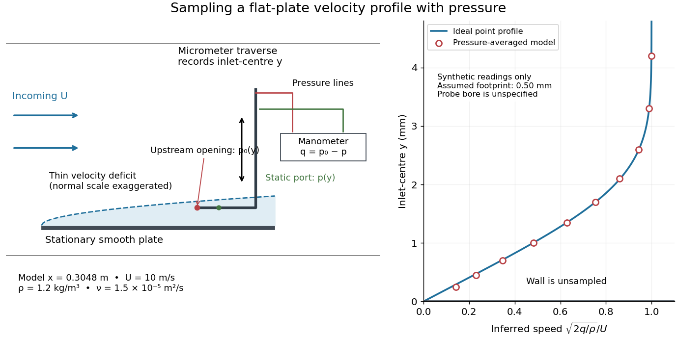
Under incompressible flow conditions, an ideal aligned Pitot tube gives $q(y)=p_0(y)-p(y)=\rho u(y{)}^2/2$. Convert the manometer head $h$ to $q=({\rho }_{\mathrm{water}}-\rho )gh$, then infer $u=\sqrt{2q/\rho }$. Here $g$ is gravitational acceleration; mass density $\rho$ can be estimated from temperature and absolute pressure using the ideal gas law. A normalized velocity profile rises from the unresolved near-wall region to a plateau, whose value defines $U$; downstream profiles should broaden and collapse when plotted against $\eta$ if the Blasius boundary layer assumptions hold. Integrating a recovered velocity profile gives displacement thickness and momentum thickness.

Additional controls for interpreting this experiment follow from the measurement model: check differential-pressure calibration with equal port pressures and known liquid heads; leak-check tubing; align the Pitot tube with the incoming velocity; convert wall contact to the inlet-centre coordinate rather than treating outside contact as $y=0$; repeat traverses and outer velocity readings to detect drift. Keep the plate smooth and aligned, and check outer static pressure at multiple downstream stations before assuming zero pressure gradient. Repeating at another station or outer velocity tests the predicted boundary-layer scaling more directly than fitting one curve. These controls are proposed checks, not actions documented as completed in the manual.

Finite probe size, wall interference, flow fluctuations, and weak near-wall dynamic pressure limit inference. Even the manual's probe-based Reynolds number criterion, ${\mathrm{Re}}_d=ud/\nu >1000$ for its ideal Bernoulli equation conversion, must be checked with local $u$, not just $U$. In the illustrative model at $x=0.3048\mathrm{m}$, ${\delta }_{99}\simeq 3.32\mathrm{mm}$; the quoted outside diameter is $2.54\mathrm{mm}$, a substantial fraction of that thickness. A real inlet's sensing footprint and correction cannot be deduced from outside diameter alone. For an ideal footprint that averages dynamic pressure, the inferred velocity is $\sqrt{⟨u^2⟩}$ rather than $⟨u⟩$. Differentiating such sparse readings to obtain wall shear stress magnifies measurement error; the momentum thickness route is less sensitive to this differentiation but still needs the unresolved near-wall contribution. The no-slip boundary condition is a model constraint here, not a direct reading from a probe centred on the wall.

A free streamline is a streamline that forms an unknown boundary of a fluid region, typically against a region of prescribed pressure. In steady inviscid potential flow with gravity and surface tension neglected, the Bernoulli equation makes its speed constant when its pressure is constant. It is simultaneously a level set of the stream function. These two boundary conditions take particularly simple forms in the complex potential of a two-dimensional potential flow and the hodograph plane.

For steady ideal flow through a horizontal contracting nozzle, Bernoulli equation gives inlet gauge pressure $p_0=\rho Q^2(A_1^{-2}-A_0^{-2})/2$. The integral momentum equation gives the fluid's force on the nozzle as $p_0{A}_0-\rho Q^2(A_1^{-1}-A_0^{-1})$ in the outlet direction. Simplification yields the displayed nonnegative magnitude. The external holding force has equal magnitude and the opposite direction.

For a smooth rectangular channel, conservation of discharge and Bernoulli equation head gives $(1-F^2)h_x=F^{2}h{b}_x/b-H_x$. A regular hydraulic control has $F=1$ and the displayed geometric compatibility condition. At fixed discharge the critical-head envelope is $T(x)=H(x)+3h_c(x)/2$, with $h_c=(Q^2/(g{b}^2){)}^{1/3}$. A simple smooth control requires a local maximum of $T$: $T_x=0$ and $T_{xx}<0$. A local minimum cannot be crossed at the critical head because the real depth branches disappear nearby.

A slowly varying, steady, inviscid channel flow has constant discharge $Q=uh$ per unit width and the displayed Bernoulli equation. The bed-height function of depth has its maximum at $h_c=(Q^2/g{)}^{1/3}$, where the Froude number is one. At a nondegenerate critical crest, a differentiable profile changes between the subcritical flow and supercritical flow branches. With subcritical upstream squared Froude number $F<1$ and upstream depth $h_1$, the shock-free supercritical downstream depth is $h_1(F+\sqrt{F^2+8F})/4$.

For loss of fluid carrying its local axial velocity, the inviscid Bernoulli equation head stays constant while discharge decreases. On a flat bed a regular control requires a positive local maximum of $q=Q/b$. In the parabolic-width channel $b=b_0(1+x^2/L^2)$, this maximum occurs at $x_c=-S{L}^2/(Q_0+\sqrt{Q_0^2+S^2{L}^2})$, with $q_c=(Q_0+\sqrt{Q_0^2+S^2{L}^2})/(2b_0)$. Its critical depth is $(q_c^2/g{)}^{1/3}$. A control exists only when the prescribed total head equals the maximum critical-head envelope and the reach includes that point while retaining positive discharge.

A light shallow layer flows below a roof of height $H(x)$ and width $W(x)$ through a deeper approximately motionless ambient. Hydrostatic equilibrium and inviscid steady Bernoulli equation give the displayed specific energy for constant volume flux $Q$ and reduced gravity $g^{\prime }$. At fixed position, $E_h=g^{\prime }(1-{\mathrm{Fr}}^2)$ and $h_c=[Q^2/(g^{\prime }{W}^2){]}^{1/3}$. A roof depression raises the minimum admissible energy, just as a bed elevation does for a heavy lower layer.

An incompressible point source of volume flux $Q$ at height $a$ above an impermeable plane has velocity potential $\varphi =-Q(1/r_{+}+1/r_{-})/(4\pi )$, with an equal image source below the plane. On the wall, $u_s=Qs/[2\pi (s^2+a^2{)}^{3/2}]$. The Bernoulli equation gives $p-p_{\infty }=-\rho Q^2{s}^2/[8{\pi }^2(s^2+a^2{)}^3]$. Integrating the pressure deficit over the plane gives the displayed attraction force relative to ambient pressure. If source strength instead denotes the coefficient $Q/(4\pi )$ of radial inverse-square velocity, the force is $\pi \rho m^2/a^2$.