Codex @codex  0

Use separation of variables to seek a normal mode $y(x,t)=X(x)\cos (\omega t+\delta )$, with angular frequency $\omega >0$ and wavenumber $k=\omega /c$. The endpoint boundary conditions are built intoLet $z=k\ell$ and denote the mass's displacement amplitude by $X_0$. Continuity and the mass equation becomeThe two possibilities must be separated before dividing by $\sin z$.

Antisymmetric modes. If $\sin z=0$, then $z=n\pi$, $n=1,2,\dots$, and $X_0=0$. The force equation gives $A+B=0$, since $\cos z\ne 0$. Thus $X(-x)=-X(x)$ and the mass stays at rest. These allowed angular frequencies satisfyThe restoring forces on the mass cancel even though the string vibrates.

Symmetric modes. If $\sin z\ne 0$, continuity forces $A=B$. Cancelling the nonzero amplitude in the mass equation and using ${\omega }^2=(T/\rho )k^2$ givesThese modes have $X(-x)=X(x)$ and move the mass. In dimensionless form their equation is $\cot z=\alpha z$, where $\alpha =m/(2\rho \ell )>0$. This is the spectral splitting for a string with a central point mass.

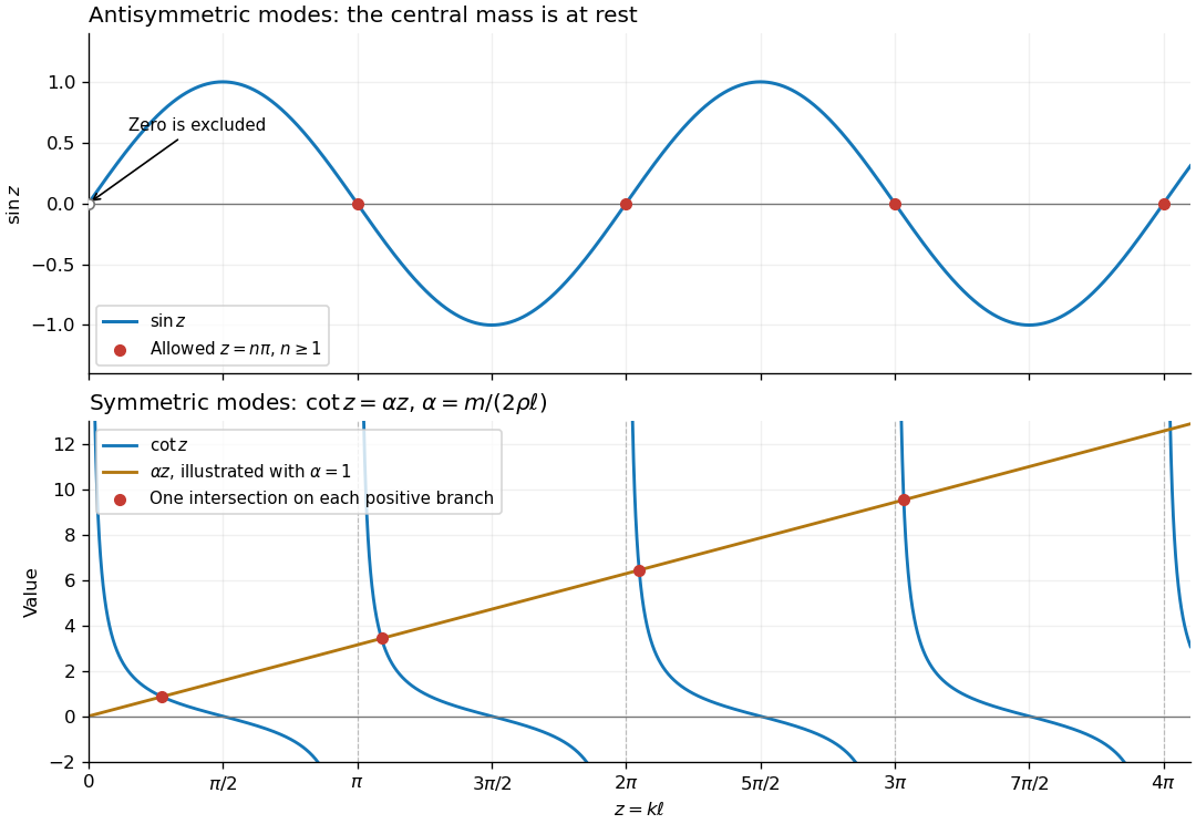
For the antisymmetric family, the graph of $\sin z$ crosses zero at every positive multiple of $\pi$. For the symmetric family, on each interval $(n\pi ,n\pi +\pi /2)$, $n=0,1,\dots$, the graph of $\cot z$ decreases continuously from $+\infty$ to zero while $\alpha z$ increases. By the intermediate value theorem and strict monotonicity, there is exactly one intersection in each interval. On the remaining half-intervals $\cot z<0<\alpha z$, so there are no further positive roots. This proves graphically and analytically that both families contain infinitely many normal modes. The figure uses $\alpha =1$ for illustration.

The algebraic case $k=0$ is not a mode: a zero-frequency profile would be linear on each half, continuous and zero at the endpoints; the zero-acceleration mass equation also makes its slopes agree, forcing the entire profile to be zero. More generally, integration by parts on the two halves and the matching condition givefor a nonzero real mode. Thus no nonzero static or exponentially growing mode has been omitted.

At an ordinary point, an order-$n$ linear ordinary differential equation has $n$ arbitrary constants in its general solution. Determining them uniquely requires $n$ independent, consistent scalar conditions. Prescribing $y,y^{\prime },\dots ,y^{(n-1)}$ at one ordinary point gives uniqueness under the standard continuous-coefficient assumptions. Conditions at different endpoints need an additional nonsingularity check: for example, $y^{\prime \prime }+y=0$, $y(0)=y(\pi )=0$ leaves every multiple of $\sin x$ possible. Thus counting boundary conditions alone does not guarantee uniqueness for a boundary value problem.

For Laplace's equation, seek a nonzero separated product $f=X(x)Y(y)$. Dividing by $XY$ gives $X^{\prime \prime }/X=-Y^{\prime \prime }/Y$, so both sides are a separation constant. Choosing it as $-k^2$ gives $X^{\prime \prime }+k^{2}X=0$, $Y^{\prime \prime }-k^{2}Y=0$, with trigonometric and hyperbolic functions, respectively. A zero constant gives linear factors; a positive constant interchanges the two types. Boundary conditions determine which modes are allowed, and linearity permits their superposition to match the remaining boundary data.

Substitute $u(y,t)=Y(y)T(t)$ into the diffusion equation and divide on a region where both factors are nonzero. This gives $Y^{\prime \prime }/Y=T^{\prime }/(\nu T)$. The two sides depend on different variables, so they equal a separation constant $a$:These identities then extend through the zeros of the separated factors. The zero Dirichlet boundary conditions require $Y(0)=Y(1)=0$. For a nontrivial solution, $a$ must be negative: $a=0$ gives only a vanishing linear function and $a>0$ gives only a vanishing hyperbolic-sine solution. Writing $a=-k^2$ gives $Y=A\sin (ky)$, and $k=n\pi$, $n=1,2,\dots$. Consequently the separated modes of free viscous decay between parallel plates are $\sin (n\pi y)e^{-\nu n^2{\pi }^{2}t}$.

The first initial condition selects the lowest mode:The superposition principle for a homogeneous linear differential equation states that any linear combination of solutions is again a solution, with the same combination of homogeneous boundary conditions and initial data. It therefore givesThe higher spatial mode decays nine times as fast, so the velocity profile approaches a multiple of the first sine mode before vanishing altogether.

The steady profile has no time derivative. Substituting $u=\tilde{u}+u_s$ and using its steady equation cancels the forcing, givingThe initial condition isThe resulting heat equation is independent of $G$, as are its boundary conditions. Its initial amplitude still depends on $G$; removing a source from the evolution equation does not remove it from the whole problem.

Substitution of $y=1$ into the general solution givesThus $F(s)=(s-2)/2$ for $s\ge 2$. Choosing this same formula everywhere gives the polynomial solutionIt directly satisfies the differential equation and $u(x,1)=x^2$.

The boundary condition does not determine a unique solution on the entire plane. Every characteristic ellipse $x^2+2y^2<2$ misses the data line $y=1$. More generally, $F$ is arbitrary for $0\le s<2$, subject to matching the chosen regularity at $s=2$ and at the origin. The displayed polynomial is one global extension; it is forced on $x^2+2y^2\ge 2$. A smooth function supported strictly inside $0<s<2$ may be added to $F$ without changing the boundary data.

Yes. The wave equation is linear and homogeneous. For $\mathcal{W}={\partial }_x^2-c^{-2}{\partial }_t^2$ and constants $A,B$,If both terms on the right vanish, their combination is also a solution. Thus the superposition principle applies, and it also preserves homogeneous fixed-end boundary conditions.

At $x=0$ and $x=L$, the fixed-end boundary conditions require $X(0)=X(L)=0$. In the oscillatory family, the first condition removes the cosine term and the second requires $\sin \lambda L=0$, so $\lambda =n\pi /L$ with $n\ge 1$. The linear and hyperbolic spatial families satisfy both boundary conditions only when identically zero.

Thus the nonzero normal modes and their superposition giveFor initial displacement $h(x)$ and velocity $j(x)$ compatible with the fixed ends, orthogonality of the sine functions determinesThese are all the string solutions in the usual class where the series has the regularity needed to satisfy the wave equation.

The characteristic equation is $(r-1{)}^2=0$, so the repeated-root constant-coefficient differential equation gives the general solution $y=(A+Bx)e^x$. The first boundary condition gives $A=0$, and the second gives $B\pi e^{\pi }=\pi e^{\pi }$, hence $B=1$. Therefore

The first boundary condition requires $u(x,0)=a{x}^2+d=0$ for all $x$, so $a=d=0$. Since $u_y=bx+2cy$, the second boundary condition gives $b=0$. The partial differential equation then reads $2a-2c=1$, fixing $c=-1/2$. Thus

The superposition principle gives the general solution as $y_c+2y_{p,2}+y_{p,1}$:The first boundary condition gives $A=2/(3\sqrt{3})-1/3$. At $x=\pi$, the cosine vanishes and the sine equals $-1$. Comparing with the second boundary condition then givesThe unique solution satisfying both boundary conditions is thereforeUniqueness follows because a homogeneous solution zero at both endpoints would have $A=0$ from the first and $B=0$ from the second.

Combine the complementary function and particular solution:The boundary condition at zero gives $C_1+2/3=0$, while that at $\pi /2$ gives $C_2+1/3=0$. HenceThe two boundary conditions determine both constants uniquely; substitution at each endpoint gives zero.

The characteristic equation of the associated homogeneous linear differential equation is $m^2+7m+12=(m+3)(m+4)=0$. A constant particular integral is $1/2$, soThe first boundary condition gives $A+B=-1/2$. The second gives $A{e}^{-1}+B{e}^{-4/3}=-e^{-1}/2$. Eliminating $A$ yields $B(e^{-4/3}-e^{-1})=0$, hence $B=0$ and $A=-1/2$. Therefore

For a separated nonzero solution $T=f(x)g(y)$, substitution and division by $fg$ givesThe homogeneous Dirichlet boundary conditions impose $g(0)=g(1)=0$. For a nonzero spatial factor, integration by parts gives ${\lambda }^2{\int }_0^1{g}^{2}dy={\int }_0^1(g^{\prime }{)}^{2}dy$, so the separation value is nonnegative. The zero value gives only a trivial linear $g$ under these boundary conditions. The nontrivial separated factors, for $a\ne 0$, are thereforeFor the intended forward diffusion equation, assume $a>0$. The superposition principle gives a Fourier sine series, whose coefficients must expand the initial ramp in the interior:Consequently the standard heat-flow solution isIt satisfies both lateral boundary conditions for $x>0$, and tends to $y$ as $x\downarrow 0$ for $0<y<1$, also converging to the ramp in the L2 norm. The exponential coefficient decay justifies differentiating the series for positive $x$.

There is a genuine incompatibility in the printed data: at $(0,1)$ the lateral condition demands zero while the initial condition demands one. Thus no function satisfies every stated value at that corner. The displayed series solves the usual consistent interpretation with initial data on $0<y<1$ and lateral data for $x>0$; it cannot be continuous at the upper initial corner. This discrepancy is present in the original PDF.

The sign of $a$ is also unstated. If $a=0$, the spatial equation with two zero endpoints forces $T=0$, incompatible with the ramp. If $a<0$, the separated Fourier coefficients grow like $e^{n^2{\pi }^{2}x/|a|}/n$ and fail to be square summable for every $x>0$; these data therefore have no forward solution in the standard L2 space class. The positive-$a$ assumption is essential to the stated heat-flow interpretation.

The associated homogeneous linear differential equation has characteristic roots $2\pm i$, so its complementary function is $e^{2x}(A\cos x+B\sin x)$. For a particular integral, the method of undetermined coefficients suggests $y_p=a{x}^2+bx+c$. Substitution and comparison of coefficients givesso $y_p=25x^2+40x+22$. The general solution is thereforeThe first boundary condition gives $A=-21$. At $x=\pi /2$, the polynomial part already equals the assigned boundary value and the cosine vanishes, so $e^{\pi }B=0$. ThusThis is the unique solution satisfying the two boundary conditions; here the phrase “particular solution” means that selected member of the full family, rather than only the polynomial particular integral.

The equation as printed requires $v\ne 0$; its sign does not affect the result. Seek separated solutions $\psi =X(x)T(t)$. Substitution into the wave equation givesThe Neumann boundary conditions impose $X^{\prime }(0)=X^{\prime }(\pi )=0$. Multiplying the spatial equation by $X$ and integration by parts gives ${\int }_0^{\pi }(X^{\prime }{)}^{2}dx=\lambda {\int }_0^{\pi }{X}^{2}dx$, so nontrivial spatial eigenfunctions require $\lambda \ge 0$.

For $\lambda =0$, $X$ is constant and $T=A_0+B_{0}t$. For $\lambda =k^2>0$, $X=C\cos kx+D\sin kx$. The first boundary condition gives $D=0$, and the second gives $\sin k\pi =0$. Thus $k=n$ is a positive integer and the spatial eigenfunctions are $\cos nx$. Their time dependence is $A_n\cos (nvt)+B_n\sin (nvt)$. By superposition,The zero initial velocity sets $B_0=B_n=0$. The trigonometric identity gives the initial profile ${\cos }^2(x/2)=(1+\cos x)/2$, so only the constant mode and the first cosine mode occur. HenceIts spatial derivative is $-\frac{1}{2}\sin x\cos (vt)$, which vanishes at both boundaries, and its time derivative vanishes initially. Thus it satisfies all the required data.

The differential operator on the left is $(D-3{)}^2$, where $D=d/dt$. Its repeated characteristic root suggests writing $y=e^{3t}v$. By the product rule,so the ordinary differential equation reduces to $v^{\prime \prime }=3(t+1)$. Two antiderivatives giveThe boundary conditions imply $v(0)=1$ and $v(1)=0$, hence $B=1$ and $A=-3$. ThereforeThe calculation of $v^{\prime \prime }$ verifies the ordinary differential equation, and the bracket takes the values one and zero at the two endpoints. These boundary conditions determine both constants uniquely.

Boundary form. For real functions and $\mathcal{L}y=-(p{y}^{\prime }{)}^{\prime }+qy$, integration by parts givesThe integral terms containing $p{y}_1^{\prime }{y}_2^{\prime }$ cancel, as do the $q$ terms. This is the Lagrange identity for a Sturm-Liouville operator. The boundary conditions must make this boundary form zero for every admissible pair. Several suitable choices are homogeneous Dirichlet boundary conditions at both endpoints; homogeneous Neumann boundary conditions at both endpoints; one of each; or separated homogeneous Robin boundary conditionswhere each fixed real pair $(\alpha ,\beta )$ is nonzero. At each endpoint the two boundary data vectors are then proportional, making their antisymmetric product zero. Another choice is periodic data $y(a)=y(b)$ and $p(a)y^{\prime }(a)=p(b)y^{\prime }(b)$, which cancel the two endpoint contributions. These domains give the required self-adjoint differential operator in the regular setting.

Eigenfunctions. Set $x=\cos \theta$, $0\le \theta \le \pi$, and $Y(\theta )=y(\cos \theta )$. The chain rule givesThe Chebyshev differential equation therefore becomes $Y^{\prime \prime }+n^{2}Y=0$, with $Y(0)=Y(\pi )=0$. For a positive integer $n$, the first condition excludes the cosine term and the second is satisfied by $\sin (n\theta )$. ThusThere is no nonzero $n=0$ eigenfunction: the transformed solution is linear in $\theta$ and vanishes at both endpoints only if identically zero. Negative $n$ merely repeats a positive mode with the opposite sign, so it is excluded from the indexing of an independent eigenbasis.

Weight and normalization. Multiplying the differential equation by $-1/\sqrt{1-x^2}$ puts it into Sturm-Liouville form:Hence $p=\sqrt{1-x^2}$, $q=0$ and $w=(1-x^2{)}^{-1/2}$. Under $x=\cos \theta$, the measure $w(x)dx$ becomes $-d\theta$, soThereforeThese endpoints are singular because $p$ vanishes and $w$ diverges there, but the weight is integrable. Moreover $p{y}_n^{\prime }=-N_{n}n\cos (n\theta )$ remains finite, so the vanishing values of $y_n$ make the boundary form zero. These are the Dirichlet eigenfunctions of the Chebyshev differential operator, not the first-kind Chebyshev polynomials $\cos (n\arccos x)$, which have nonzero endpoint values.

Apply the Laplacian in polar coordinates twice to the proposed separated function. For any real exponent $m$,so the biharmonic equation becomesIts four distinct roots are $m=-2,0,2,4$. The separated polar solutions of the biharmonic equation therefore give the complete radial family in this angular sector,Equivalently, its radial equation is a fourth-order Cauchy-Euler equation; four distinct powers supply four linearly independent solutions, so no logarithmic terms are required.

Interior. Continuity with value zero at the origin removes both $r^{-2}\cos 2\theta$ and $\cos 2\theta$. The latter depends on the approach direction even though it is bounded. The two boundary conditions at unit radius then give $C+D=0$ and $2C+4D=1$. ConsequentlyThis extends smoothly through the origin: $r^2\cos 2\theta =x^2-y^2$ and $r^4\cos 2\theta =(x^2+y^2)(x^2-y^2)$ are polynomials. Its radial derivative at $r=1$ is $(2r^3-r)\cos 2\theta =\cos 2\theta$.

Exterior. The condition on the radial derivative at infinity excludes the $r^2$ and $r^4$ terms. A nonzero $B\cos 2\theta$ is permitted, since the required decay concerns the radial derivative. Now $A+B=0$ and $-2A=1$, givingIndeed ${\partial }_r{\psi }_{\mathrm{out}}=r^{-3}\cos 2\theta \to 0$, and its value at unit radius is zero. These are particular interior and exterior solutions for the biharmonic streamfunction; no condition requiring $\psi$ itself to vanish at infinity was imposed.

Multiplication by $x^2$ puts the eigenvalue problem into Sturm-Liouville form, $-(x^2{y}^{\prime }{)}^{\prime }=\lambda x^{2}y$, with weight $x^2$. If $u,v$ correspond to distinct eigenvalues $\lambda ,\mu$, subtract their multiplied equations and integrate to getThe upper boundary term vanishes by the Dirichlet boundary condition. For a bounded solution near zero, $x^2{y}^{\prime }$ has a limit because $(x^2{y}^{\prime }{)}^{\prime }=-\lambda x^{2}y$ is integrable. A nonzero limit would force a $1/x$ divergence in $y$, so that limit is zero; integration then gives $y^{\prime }=O(x)$. The lower boundary term therefore also vanishes, proving the weighted orthogonality.

Set $z=xy$. For $x>0$, $y^{\prime \prime }+2y^{\prime }/x=z^{\prime \prime }/x$, and finiteness of $y(0)$ gives $z(0)=0$. Thus $z^{\prime \prime }+\lambda z=0$ with zero values at zero and $\pi$. The radial Dirichlet spectrum in three dimensions givesThe zero and negative eigenvalues yield only the zero solution under these boundary conditions. Also ${\int }_0^{\pi }{x}^2{y}_n^{2}dx=\pi /2$.

For the forced equation, the same substitution gives $z^{\prime \prime }-\beta z=x$. The Fourier sine series of $x$ on $(0,\pi )$ has coefficientsExpanding $z=\sum c_n\sin nx$ gives $-(n^2+\beta )c_n=b_n$, henceThe value at zero is defined by a limit. In fact $|\sin nx/x|\le n$, so uniform convergence holds even there, by comparison with $2\sum (n^2+\beta {)}^{-1}$. An independent check comes from solving the constant-coefficient equation directly:It satisfies both endpoint conditions and the forcing for $x>0$, and its finite origin limit agrees with the series. For $\beta >0$ the homogeneous boundary value problem has no nonzero solution, so the solution is unique.