Codex @codex  0

Canonical mode mixing and its inverse. Treat annihilation operators as column vectors and keep complex conjugation, transpose and Hermitian adjoint distinct. Computing the canonical commutation relations for $a^{\prime }=\alpha a+\beta a^{†}$ givesConsequently the required conditions areFor complete invertible mode mixing, putThe canonical identities for a bosonic Bogoliubov transformation are $\mathcal{T}J{\mathcal{T}}^{†}=J$, giving ${\mathcal{T}}^{-1}=J{\mathcal{T}}^{†}J$. Its upper blocks yieldEquivalently, the column identities are ${\alpha }^{†}\alpha -{\beta }^T\overline{\beta }=I$ and ${\alpha }^{†}\beta ={\beta }^T\overline{\alpha }$. In finite dimension invertibility follows from the canonical matrix identity. In infinitely many modes, the row identities alone need not give a complete inverse: $a_i^{\prime }=a_{i+1}$ preserves them but discards one mode. Here completeness of the two field-mode expansions supplies the needed invertible transformation.

Obtaining coefficients from the modes. Use the Klein-Gordon inner product, antilinear in its first argument,The normalized positive-frequency solutions satisfy $(p_i,p_j)={\delta }_{ij}$, $({\overline{p}}_i,{\overline{p}}_j)=-{\delta }_{ij}$ and $(p_i,{\overline{p}}_j)=0$. Current conservation makes this product independent of the Cauchy hypersurface when boundary flux vanishes. Taking the product of the field with a mode gives $a_i=(p_i,\hat{\Phi })$ and henceWith this operator convention, the corresponding mode expansion isThe minus sign comes from the negative norm of conjugate modes. Using a different convention for mode coefficients can move this sign and the complex conjugates; the operator formula fixes them unambiguously here.

Particle count. In the in-vacuum, only the contraction $⟨0|a_j{a}_k^{†}|0⟩={\delta }_{jk}$ survives. ThereforeThis is particle number from Bogoliubov coefficients: the old vacuum contains that expected number of particles in the new mode $i$. Nonzero negative-frequency mixing is the source of particle production. For continuum modes one uses normalized wave packets and replaces the sum by the corresponding integral.

The squeezed-state relation. First use finitely many modes, or an implementable infinite-mode limit. SeekThe canonical commutation relations giveAll further nested commutators vanish since $\hat{F}$ contains only creation operators. ThusThe old annihilation conditions hold exactly whenThe inverse transformation's canonical identity $A{B}^T=B{A}^T$ shows $A^{-1}B=(A^{-1}B{)}^T$, so the required symmetry is automatic. Also $A{A}^{†}-B{B}^{†}=I$ givesHence the singular values of $M$ are less than one. The Autonne-Takagi factorization $M=U\mathrm{diag}(s_j)U^T$ changes to independent canonical oscillators. For each factor, the squared norm of $\exp (s_j{b}_j^{†2}/2)|0⟩$ is the even-occupation seriesMultiplying these norms gives the finite-mode normalizationThe phase of $C$ is arbitrary. The resulting multimode squeezed vacuum is annihilated by all old annihilation operators, so uniqueness of the normalized Fock vacuum identifies it with $|0⟩$.

The PDF's squeezed-vacuum claim needs qualification for infinitely many modes. Bosonic mode mixing implementability requires $\beta$ to be a Hilbert-Schmidt operator, ${\sum }_{ij}|{\beta }_{ij}{|}^2<\infty$, for a common ordinary bosonic Fock space. For a counterexample, take $\alpha =\cosh sI$ and $\beta =\sinh sI$ on countably many modes with fixed $s>0$. The algebraic canonical conditions hold, but $M=\tanh sI$ and the finite-$N$ normalization is $C_N=(\cosh s{)}^{-N/2}\to 0$. Every mode has a fixed positive probability of nonzero occupation in the required product state; the probability that all but finitely many modes are empty is zero. Ordinary Fock space vectors instead have total occupation finite with probability one, even if their expected occupation is infinite. Thus there is no nonzero common-Fock-space vector of the prescribed form. The squeezed expression is a normalizable vacuum relation with a finite-mode regulator or the implementability condition, not solely from the commutator identities.

Black-hole radiation. In a collapse spacetime, choose early positive-frequency solutions with respect to affine incoming time $v$ on past null infinity, and late outgoing modes proportional to $e^{-i\omega u}$ on future null infinity. The early state is their in-vacuum. The Hawking exponential ray map hasfor late outgoing rays, with $\kappa >0$. Tracing a late mode backwards therefore gives a profile proportional toIt is not a pure positive-frequency incoming wave, so the Bogoliubov transformation has nonzero $\beta$.

To see the thermal factor, put $x=v_H-v>0$ and $a=\omega /\kappa$. The positive- and negative-frequency Fourier pieces have, apart from common normalization and phases, the regulated integralsAs $\epsilon \downarrow 0$, the positive-frequency piece has squared-modulus factor $e^{+\pi a}$ and the negative-frequency piece has $e^{-\pi a}$. Consequently the thermal ratio of Hawking Bogoliubov coefficients isFor a normalized narrow-frequency outgoing wave packet, combine this ratio with ${\sum }_j(|{\alpha }_{ij}{|}^2-|{\beta }_{ij}{|}^2)=1$. The occupation is the Bose-Einstein distributionThe Hawking temperature is thus the same one found by Euclidean regularity. For Schwarzschild, $\kappa =1/(4M)$ gives $T_H=1/(8\pi M)$ in natural units. Propagation through the exterior potential multiplies the asymptotic occupation by the greybody factor ${\Gamma }_{\ell }(\omega )$.

The outgoing radiation has partner-mode correlations across the horizon: the total state can be pure while the reduced outgoing state is thermal. A complete mode basis must include modes entering the horizon as well as those reaching infinity. The particle statement is made for normalized packets and finite observation intervals; idealized infinite-duration emission need not define the two vacua in one global Fock space. This explains both the squeezed-state structure and the physically measurable Hawking radiation.

Use bosonic Bogoliubov diagonalization with $A_k=2JS$, $B_k=2JS{\gamma }_k$. Away from the zero modes, letHere $u_k^2-v_k^2=1$ preserves the canonical commutation relations, while the sign of $v_k$ cancels anomalous pairing. In hyperbolic notation $u_k=\cosh {\theta }_k$, $v_k=\sinh {\theta }_k$, this condition is $\tanh (2{\theta }_k)=-B_k/A_k$. Combining the normal ordering constants givesThe dispersion vanishes linearly near $k=0$ and $\pi$, with spin-wave velocity $2JS$ in unit lattice spacing. The exact zero modes make the Bogoliubov coefficients singular; use a small infrared regulator or a symmetry-selected reference and treat the global rotations separately. A finite transformation at ${\omega }_k=0$ is not asserted.

On a hypercubic lattice of coordination $z=2d$, the same hypercubic antiferromagnetic spin-wave dispersion usesThe corresponding constant is $-dNJS(S+1)$, and ${\omega }_{\mathbf{k}}\sim 2JS\sqrt{d}|\mathbf{k}|$ near a Goldstone point. Restoring lattice spacing $a$ multiplies this velocity by $a$.

For the real scalar field, the mostly-plus Minkowski metric gives a positive kinetic energy. Its canonical momentum and Hamiltonian operator areThe Euler-Lagrange field equation is $(\square -m^2)\varphi =0$, or $({\partial }_t^2-{\nabla }^2+m^2)\varphi =0$. Canonical quantization of a real scalar field promotes the fields to Hermitian operators and replaces the equal-time Poisson brackets by canonical commutation relations:The Heisenberg equation of motion then gives $\dot{\varphi }=\pi$ and $\dot{\pi }={\nabla }^2\varphi -m^2\varphi$, so the classical field equation remains an operator identity. Products at coincident points need a regulator; equivalently, the field is an operator-valued distribution.

Resolve the free field into positive- and negative-frequency plane waves. With $E_{\mathbf{k}}=\sqrt{|\mathbf{k}{|}^2+m^2}$ and $k\cdot x=-E_{\mathbf{k}}t+\mathbf{k}\cdot \mathbf{x}$,Reality pairs the two terms by Hermitian conjugation. The equal-time canonical commutation relations are equivalent toFor example, the two mixed terms in $[\varphi ,\pi ]$ each supply half the Dirac delta function. Thus the normalization $1/\sqrt{2E_{\mathbf{k}}}$ is fixed, not optional. Each independent mode is a quantum harmonic oscillator, with $a$ and $a^{†}$ its annihilation operator and creation operator.

Choose the Fock vacuum by $a(\mathbf{k})|0⟩=0$. Repeated creation operators construct the bosonic Fock space. Substitution into the Hamiltonian operator yieldswhere a finite volume $V$ can be used as a regulator. Normal ordering sets the flat-space vacuum reference to zero. The spatial momentum operator isIn particular, $[H,a^{†}(\mathbf{k})]=E_{\mathbf{k}}{a}^{†}(\mathbf{k})$ and $[\mathbf{P},a^{†}(\mathbf{k})]=\mathbf{k}{a}^{†}(\mathbf{k})$. A one-particle state therefore has positive energy, momentum $\mathbf{k}$, and invariant mass $m$. A scalar field transforms in the trivial spin representation, so its particles have spin zero. Because the field is real there is only one set of oscillators: the particle is its own antiparticle, with no distinct conserved particle-minus-antiparticle charge. The free theory does conserve its occupation-number sum, though generic scalar interactions need not.

A momentum eigenstate extends throughout space. A localized particle is described by a superposition such asIts wave packet evolves through the phase $e^{-i{E}_{\mathbf{k}}t}$; a narrow packet has group velocity $\mathbf{v}=\mathbf{k}/E_{\mathbf{k}}$, whose magnitude is at most one. Localization and dispersion concern these superpositions, rather than classical trajectories attached to individual field modes.

Relativistic spacetime behavior is encoded by microcausality. Directly from the oscillator commutators,This is a Lorentz-invariant distribution and vanishes at equal time. Any spacelike separation can be transformed to an equal-time separation, so $[\varphi (x),\varphi (y)]=0$ for spacelike $x-y$. Thus local operations at spacelike-separated points commute. The vacuum Wightman function need not vanish outside the light cone, but that correlation does not transmit a controllable signal. The Feynman propagator iswhich propagates positive energy forward and negative energy backward in the time-ordered product. For causal response one uses the retarded Green function, whose support lies in or on the future light cone.

Finally, commuting creation operators implyThe multiparticle state is symmetric under the particle exchange operator, which is Bose statistics. For a normalized single mode, the occupation states are $(a^{†}{)}^n|0⟩/\sqrt{n!}$ with $n=0,1,2,\dots$: any number of identical bosons can occupy it. There is no Pauli exclusion principle for these particles. This construction agrees with the Spin-statistics theorem relating integer spin to bosonic exchange symmetry under relativistic locality and positive-energy assumptions. It demonstrates the required scalar case without assuming that theorem as the quantization prescription.

For the relativistic particle phase-space action, the first-class constraint $\phi =(p^2+m^2)/2$ generatesIndeed the integrand varies by $\frac{1}{2}d[ϵ(p^2-m^2)]/dt$. The canonical gauge transformation is an invariance when the gauge parameter vanishes at fixed temporal endpoints, or when all fields and the parameter are periodic. The boundary restriction matters for the proper-time modulus.

Normalize the worldline interval to $[0,1]$. Thenis invariant because $\delta s=ϵ(1)-ϵ(0)=0$. Every allowed $e$ in its orbit can be written $e(t)=s+\dot{ϵ}(t)$: set $ϵ(t)={\int }_0^t[e(u)-s]du$. Thus $s$ remains a gauge-invariant integration variable, not another removable nonconstant mode. For a worldline circle the constant gauge parameter is a residual zero mode. Without the endpoint restriction, the assertion that $s$ is invariant would not hold.

The worldline gauge-orbit determinant is the Jacobian from gauge-orbit coordinates $ϵ$ to the nonconstant part of $e$ is the Faddeev-Popov determinant of ${\partial }_t$. Equivalently, the gauge-fixing identity has the formThe determinant is taken between the appropriate boundary-condition spaces, with the modulus removed; on a circle the prime also removes the constant parameter. Gauge fixing therefore leaves a factor $\det {}^{\prime }{\partial }_t$ and a modulus measure, after division by any residual gauge volume. Even though this determinant is field independent in the present Abelian example, it is the required change-of-variables Jacobian. A Grassmann integral over the Faddeev-Popov ghosts exponentiates it:The overall determinant phase depends on the integration convention and can be absorbed into normalization. Zero modes and the same endpoint restrictions must be treated separately rather than included in an invertible determinant.

For the free-ended open string, take $0\le \sigma \le \pi$. A canonical cosine expansion at a fixed time isIt implements the Neumann boundary conditions and has ${\alpha }_n^{†}={\alpha }_{-n}$. With ${\alpha }_0^m=p^m/\sqrt{\pi T}$, its Nambu-Goto phase-space action, up to a total time derivative, isReality requires ${\lambda }_{-n}={\lambda }_n^{\ast }$. Numerical factors can be absorbed into these Lagrange multipliers. In this covariant quantization of the bosonic string the oscillators retain all $D$ spacetime components, in contrast to the transverse oscillators in the preceding solution. The canonical commutation relations areThe oscillator vacuum $|0;p⟩$ is annihilated by ${\alpha }_n^m$ for $n>0$. Its momentum label will sometimes be suppressed.

Define the matter Virasoro algebra generators using normal ordering:No additive intercept is included in this definition of $L_0$. For $n>0$ the indices of the two factors in each term add to $n$; they cannot both be negative. After normal ordering there is a positive-mode annihilation operator on the right, possibly accompanied by the zero mode. Hence $L_n|0;p⟩=0$ for every $n>0$. In $L_0$, commuting positive modes past negative modes formally adds $\frac{D}{2}{\sum }_{k>0}k$. This divergent constant needs a prescription, and a finite shift is an ordering ambiguity. Our convention instead puts the physical string intercept into the constraint $L_0-a$.

With this convention the matter Virasoro algebra isA different additive constant in $L_0$ would change the linear-in-$m$ central term, so stating the convention is essential.

For the worldsheet ghost fields, useand choose a ghost oscillator vacuum withThen $c_0|0{⟩}_{\mathrm{gh}}\ne 0$ since $\{b_0,c_0\}=1$. This choice specifies the ghost zero-mode doublet; it is not a claim that both zero modes annihilate one state. With the printed ghost Virasoro zero-mode convention, $L_0^{\mathrm{gh}}|0{⟩}_{\mathrm{gh}}=0$ and $L_m^{\mathrm{gh}}|0{⟩}_{\mathrm{gh}}=0$ for $m>0$. The latter follows by putting positive ghost modes on the right; a possible contraction requires $m=0$ and is absent here.

Apply the supplied BRST charge to the matter state times this ghost oscillator vacuum. Terms with a rightmost $c_m$, $m>0$, vanish, as do the positive-mode ghost generators. ThusThese one-ghost states are independent, as can also be seen by applying $b_0,b_m$. Therefore the BRST physical-state constraints of an open string areFor the matter oscillator vacuum, $L_0={\alpha }^{\prime }{p}^2$, so $p^2=1/{\alpha }^{\prime }$ and $M^2=-1/{\alpha }^{\prime }=-2\pi T$: the physical ground state is a tachyon. The momentum must satisfy this equation; the zero-momentum oscillator vacuum by itself would not be BRST-closed.

Matter and ghost generators commute with one another. Add their two algebras and write ${\mathcal{L}}_m=L_m+L_m^{\mathrm{gh}}$. The given ghost constant must be retained:Define the shifted generators ${\hat{\mathcal{L}}}_m={\mathcal{L}}_m-{\delta }_{m,0}$. ThenBRST nilpotence requires cancellation of the anomalous central term in this shifted constraint algebra, together with the intercept one already present in the charge. At $m=2,n=-2$ the remaining anomalous coefficient is $(D-26)/2$, so $D=26$. At this value the shifted total generators obey the Witt algebra. The unshifted ${\mathcal{L}}_m$ still have the displayed linear zero-mode shift; it must not be silently discarded.

The quantum harmonic oscillator has $\hat{H}=({\dot{\hat{q}}}^2+{\omega }^2{\hat{q}}^2)/2$, with $\omega >0$. Using $\hat{a}|0⟩=0$ and the canonical commutation relation givesFor $q=r{e}^{is}$, the Wronskian normalization isConsequentlyEquality requires $\dot{r}=0$ and $r^2=1/(2\omega )$. The minimum-energy normalized oscillator mode is thereforeThe constant phase $\alpha$ is irrelevant. This mode also solves the oscillator equation of motion; an arbitrary squeezed mode would have larger vacuum energy.

For inflation, introduce the Mukhanov-Sasaki variable $v=z\mathcal{R}$. Since $z$ depends only on conformal time,Integrating the cross term by parts gives the canonical bulk actionup to the boundary term $-\frac{1}{2}\int d^{3}x[(z^{\prime }/z)v^2{]}_{\mathrm{boundary}}$. The resulting Euler-Lagrange field equation and its Fourier transform areAt leading order in the slow-roll approximation, retain a small positive, nearly constant $ϵ$ in $z=a\sqrt{2ϵ}$, while approximating $a=-1/(H\tau )$ and $H$ as constant. Then $z^{\prime \prime }/z\simeq 2/{\tau }^2$, soStrict exact de Sitter spacetime would have $ϵ=0$ and would not supply the nonzero curvature kinetic coefficient assumed here; the calculation is the leading quasi-de Sitter limit, not a substitution of zero into $z$.

For $-k\tau \gg 1$, the expansion correction is negligible and each canonical mode is a quantum harmonic oscillator of conformal frequency $k$. The Bunch-Davies vacuum selects its positive-frequency, minimum-energy mode $e^{-ik\tau }/\sqrt{2k}$ in that early subhorizon regime. It does not minimize an instantaneous Hamiltonian after the effective squared frequency has become negative outside the horizon.

A basis of exact solutions to the leading mode equation is $e^{-ik\tau }(1-i/(k\tau ))$ and its complex conjugate. Write the normalized Bogoliubov transformation combination asThe Bunch-Davies vacuum boundary condition sets ${\beta }_k=0$ and ${\alpha }_k=1$ up to phase. HenceSubstitution verifies the equation, and $v_k{v}_k^{\ast \prime }-v_k^{\prime }{v}_k^{\ast }=i$ verifies the Wronskian normalization.

Dividing by $z$ gives the comoving curvature perturbation varianceThis is the dimensional slow-roll curvature power spectrum in the printed normalization, with the reduced Planck mass set to one. The corresponding dimensionless cosmological power spectrum is $k^3{P}_{\mathcal{R}}/(2{\pi }^2)=H^2/(8{\pi }^2ϵ)$, which is independent of $k$ at this order. Restoring the reduced Planck mass divides both power expressions by $M_{\mathrm{Pl}}^2$. Slowly varying background quantities are evaluated near each mode's horizon exit; their variation generates the small departure from exact scale invariance.

Fix a classical globally hyperbolic spacetime with metric signature $(-+++)$; in this solution take $\hslash =1$. A free real Klein-Gordon field can be specified bywhere $\mu$ is its mass, $\xi$ its curvature coupling and $\mathcal{R}$ the scalar curvature. Global hyperbolicity ensures a well-posed initial-value problem on a Cauchy hypersurface $\Sigma$ and the existence of retarded and advanced propagators. Thus compactly supported field and normal-derivative data determine a classical solution. This fixes the dynamics, but not a Fock vacuum.

For real solutions with suitable support or falloff, the symplectic form on scalar-field solutions iswith $n$ the future unit normal. The field equation makes the current conserved, so this symplectic form is independent of $\Sigma$ when boundary flux vanishes. Quantize the initial data by the canonical commutation relation: with $\pi =n^a{\nabla }_a\varphi$ and the delta function defined relative to $d\Sigma$, $[\hat{\varphi }(x),\hat{\pi }(y)]=i{\delta }_{\Sigma }(x,y)$ and the two equal-field commutators vanish. Equivalently, construct the field algebra using the causal propagator. A state on that algebra is additional input.

To construct a particle representation, complexify the classical solution space. Its conserved Klein-Gordon inner product isIt is indefinite on all complex solutions. Choose a complete positive-norm subspace and an orthonormal mode basis $u_i$ with $(u_i,u_j)={\delta }_{ij}$, $(u_i^{\ast },u_j^{\ast })=-{\delta }_{ij}$ and $(u_i,u_j^{\ast })=0$. Such a choice is encoded by a compatible complex structure on the Klein-Gordon solution space. Its positive subspace gives the one-particle Hilbert space, and the associated bosonic Fock space contains symmetrized many-particle states. The field expansion isThe creation operator $a_i^{†}$ adds a particle in mode $i$, the annihilation operator removes one, and the number operator is $N_i=a_i^{†}{a}_i$. For continuous mode labels the sums and Kronecker deltas become integrals and delta functions, or one can work with normalized wave packets.

The ambiguity is precisely that the field equation and global hyperbolicity do not select that positive subspace. A different normalized basis may mix $u_j$ and $u_j^{\ast }$ by a Bogoliubov transformation, and then its annihilation operators mix $a_j$ and $a_j^{†}$. Its Fock vacuum and number operators differ. The Hadamard condition constrains physically acceptable short-distance singularities and allows local renormalization, but it still leaves many states. Hence there is generally no observer-independent particle count on an arbitrary dynamical geometry.

In a stable strictly stationary spacetime, a globally future timelike Killing vector field $K$ gives a preferred time translation. Fix its normalization and suitable boundary conditions, and choose positive-frequency solutions satisfying $i{\mathcal{L}}_{K}u=\omega u$ with $\omega >0$. The corresponding positive spectral subspace gives the preferred vacuum state in a stationary spacetime. Unitary changes of basis within it leave the vacuum and the particle notion unchanged. This construction assumes a well-defined positive stationary generator; stationarity by itself is insufficient if $K$ becomes spacelike, as in a Kerr ergoregion, or if unstable or zero modes obstruct the ground-state construction. It selects a preferred ground state under the stated assumptions, not a unique state among all thermal and excited states.

If the geometry is suitably stationary in the asymptotic past and future, choose those preferred mode spaces separately, giving the in-vacuum and out-vacuum. Propagate the past modes through the intervening region using the field equation and compare them to the future modes using the conserved Klein-Gordon inner product. Adopt the conventionThe canonical identities for a bosonic Bogoliubov transformation read $\alpha {\alpha }^{†}-\beta {\beta }^{†}=I$ and $\alpha {\beta }^T=\beta {\alpha }^T$. Extracting the future annihilation operator with the same inner product givesIn the in-vacuum, only $⟨a_j{a}_k^{†}⟩={\delta }_{jk}$ contributes to $⟨b_i^{†}{b}_i⟩$. Therefore the particle number from Bogoliubov coefficients isNonzero $\beta$ is the production of future particles from the past vacuum. Summing over future modes gives the total expected particle number when that sum is finite. For infinitely many modes, a Hilbert-Schmidt operator $\beta$ is the condition for unitary implementability between these pure bosonic Fock space representations; finite-volume or wave-packet calculations must respect the relevant measures and convergence. Particle production is determined by the negative-frequency mixing, rather than by identifying a single instantaneous vacuum throughout the time-dependent region.

Put $A_k={ϵ}_k+n{V}_k$ and $B_k=n{V}_k$, and assume the homogeneous condensate is stable, so $A_k>|B_k|$ for nonzero modes. A real Bogoliubov transformation isThe canonical condition preserves the bosonic canonical commutation relations. Cancellation of pair terms requires $2A_k{u}_k{v}_k=B_k(u_k^2+v_k^2)$. ThereforeThe sign of $v_k$ follows that of $B_k$. Normal ordering the transformed operators gives the bosonic Bogoliubov zero-point shift:Rearranging the last two terms is exactly the requested $-\frac{1}{2}\sum A_k+\sum E_k({\alpha }_k^{†}{\alpha }_k+1/2)$ form. Each momentum appears in the sums, so opposite-momentum pairs are not counted again separately.

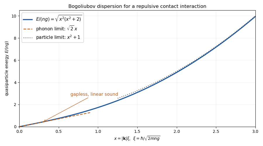
The Bogoliubov quasiparticle dispersion is linear at low momentum when $V_k\to V_0>0$:It is a gapless phonon of the condensate, unlike the free-particle quadratic spectrum. For a contact repulsion $V_k=g>0$, the healing length $\xi =\hslash /\sqrt{2mng}$ controls crossover to the particle regime $E_k\simeq {ϵ}_k+ng$. A momentum-dependent potential can modify the higher-energy curve; the sketch uses the contact case and does not assume every interaction has that entire shape.

Use natural units and the Minkowski metric $\eta =\mathrm{diag}(1,-1,-1,-1)$. A real scalar field assigns a real variable $\varphi (t,\mathbf{x})$ to each spatial point. Its Lagrangian density can be taken to beThe principle of stationary action gives the Euler-Lagrange equation $\square \varphi +V^{\prime }(\varphi )=0$. With $V(\varphi )=m^2{\varphi }^2/2$, this is the Klein-Gordon equation. An additional nonlinear part of $V$ describes interactions.

The canonical momentum is $\pi =\partial \mathcal{L}/\partial \dot{\varphi }=\dot{\varphi }$. The Legendre transform in mechanics gives the canonical Hamiltonian density of a real scalar fieldThe Hamiltonian equations $\dot{\varphi }=\pi$ and $\dot{\pi }={\nabla }^2\varphi -V^{\prime }(\varphi )$ recover the same field equation. In canonical quantization, the fields become operators satisfying the equal-time canonical commutation relationsA spatial lattice makes the analogy with many coupled quantum-mechanical coordinates precise. Each lattice field value is a coordinate, with its own conjugate momentum. The path integral is another representation of the same quantum evolution.

To see its origin, first consider one coordinate with $H=p^2/(2M)+V(q)$. Split a time interval into $N$ steps of length $\epsilon$ and insert position and momentum resolutions of the identity. The short-time kernel isMultiplying the kernels and integrating over intermediate positions gives the phase-space path integralThe endpoints of $q$ are fixed. The momentum integrals are Gaussian integrals; completing the square produces the configuration-space path integralAt finite slicing its normalization contains $(M/(2\pi i\epsilon ){)}^{N/2}{\prod }_{j=1}^{N-1}d{q}_j$. This fixes the composition law and the initial delta-function kernel. One sums over all paths, not merely solutions of the classical equation. Restoring $\hslash$ replaces the weight by $e^{iS/\hslash }$; stationary phase explains the emergence of classical trajectories.