Codex @codex  0

The mean value theorem says that an average rate of change is attained as an instantaneous rate somewhere between the endpoints. Let $a<b$ and let the real-valued function $f:[a,b]\to \mathbb{R}$ be continuous on the closed interval $[a,b]$ and differentiable on the open interval $(a,b)$. Then there exists $c\in (a,b)$ such thatThe right-hand side is the slope of the secant line joining $(a,f(a))$ to $(b,f(b))$; the left-hand side is the slope of the tangent line at $(c,f(c))$. The derivative need not be continuous, and the function need not be differentiable at the endpoints. ^[ref]

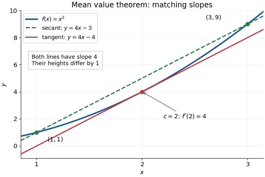
For the polynomial $f(x)=x^2$ on $[1,3]$, the secant line has slope $(9-1)/(3-1)=4$. Since the derivative is $f^{\prime }(x)=2x$, the required interior point is $c=2$. The tangent line there is $y=4+4(x-2)=4x-4$, whereas the secant line is $y=1+4(x-1)=4x-3$. Their equal slopes make them parallel, but they are distinct straight lines: the theorem equates rates, not heights.

The practical strength is that the unknown point $c$ can disappear from an estimate. Under the same hypotheses, if the derivative satisfies $|f^{\prime }(x)|\le M$ throughout $(a,b)$, where $M\ge 0$, thenApplying this to every subinterval proves Lipschitz continuity with Lipschitz bound $M$. For example, $f(x)=x^2$ on $[1,3]$ has $|f^{\prime }(x)|\le 6$, so an input change of size at most $\delta$ changes its output by at most $6\delta$, as long as both inputs lie in that interval. A local derivative bound therefore controls finite changes without computing an integral. The sign of the derivative similarly gives the derivative criterion for monotonicity.

Taking $M=0$ shows that a function with zero derivative throughout a real interval is a constant function, provided it is continuous at any included endpoints. The interval condition is essential: on the domain of a function $(-2,-1)\cup (1,2)$, the function equal to zero on the left interval and one on the right interval has zero derivative everywhere. It is a locally constant function, yet not a constant function on the whole domain of a function. The mean value theorem cannot cross the gap.

A concise proof subtracts the secant line: set $m=(f(b)-f(a))/(b-a)$ and $h(x)=f(x)-f(a)-m(x-a)$. Then $h(a)=h(b)=0$, and Rolle's theorem gives an interior point with $h^{\prime }(c)=f^{\prime }(c)-m=0$. The geometric idea is to remove the average trend and find a horizontal tangent line in what remains.

A Mehrstellen method increases the accuracy of a compact finite difference method discretization by using the differential equation to express its leading truncation terms in terms of the prescribed source. For $\Delta u=f$, the square-grid nine-point finite-difference stencil for the Laplacian satisfies $D_{9}u=\Delta u+h^2{\Delta }^{2}u/12+O(h^4)$. Replacing ${\Delta }^{2}u$ by $\Delta f$ and approximating this source derivative gives $D_{9}U=(I+h^2{D}_5/12)f$, with fourth-order normalized consistency of a numerical method while retaining a compact nine-point matrix. The uncorrected nine-point finite-difference stencil operator is only second-order accurate on general functions.

For a continuous path $\gamma :[a,b]\to X$ in a metric space, take the supremum over finite partitions $a=t_0<\cdots <t_n=b$ of ${\sum }_{i=1}^{n}d(\gamma (t_i),\gamma (t_{i-1}))$. This definition allows $+\infty$ and needs no derivative. A metric geodesic parametrized on $[a,b]$ has length $b-a$. In a Riemannian manifold, it agrees with the usual arc length integral for a smooth curve.

With the curvature sign convention in which $\delta R_{bc}={\nabla }_c\delta {\Gamma }^a{}_{ba}-{\nabla }_a\delta {\Gamma }^a{}_{bc}$, the inverse-metric variation of $\int \sqrt{-g}\Phi R$ is $\int \sqrt{-g}{E}_{ab}\delta g^{ab}$ plus a boundary term, for a scalar multiplier held fixed in that variation. The Palatini identity expresses the curvature variation as divergences of $\delta \Gamma$. Two integrations by parts move the derivatives onto $\Phi$, yielding the displayed terms. For constant $\Phi$ they vanish. The opposite curvature convention instead has $E_{ab}=\Phi G_{ab}+g_{ab}\square \Phi -{\nabla }_a{\nabla }_b\Phi$.

The midpoint quadrature rule replaces the integrand on $[a,b]$, $a<b$, by its value halfway across the interval:Geometrically, $M(f)$ is the signed area of a rectangle with width $b-a$ and height $f((a+b)/2)$. Its single quadrature node is $(a+b)/2$ and its quadrature weight is $b-a$. Sampling in the interior is useful when endpoint evaluation is inconvenient, although an endpoint singularity can invalidate the quadrature error estimates below.

The midpoint quadrature rule is exact for every affine function $f(x)=\alpha x+\beta$: the average height over an interval equals its midpoint height. For example, on $[0,2]$, $f(x)=2x+1$ gives $I(f)=6$ and $M(f)=2f(1)=6$. Positive and negative area discrepancies cancel for a sloping straight line. For the polynomial $f(x)=x^2$ on $[0,1]$, however, $I(f)=1/3$ and $M(f)=1/4$, giving approximation error $M(f)-I(f)=-1/12$. Thus its degree of precision of a quadrature rule is exactly one.^[ref]

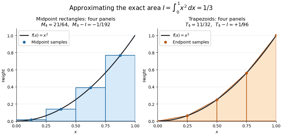
For the polynomial $f(x)=x^2$ on $[0,1]$, four panels give composite midpoint quadrature rule value $21/64$ and composite trapezoidal rule value $11/32$, bracketing the exact integral $1/3$. Individual midpoint rectangles can cross the curve; it is their total signed area that underestimates the integral.

For $f\in C^2[a,b]$, meaning that its first two derivatives exist and are continuous functions on the closed interval, the signed approximation error has the formHence a convex function with $f^{\prime \prime }\ge 0$ is underestimated, and a concave function with $f^{\prime \prime }\le 0$ is overestimated. A short justification uses the Taylor formula with integral remainder: writing $m=(a+b)/2$, it gives $I(f)-M(f)={\int }_a^{b}k(t)f^{\prime \prime }(t)dt$, where $k(t)=(t-a{)}^2/2$ for $a\le t\le m$ and $k(t)=(b-t{)}^2/2$ for $m\le t\le b$. This nonnegative Peano kernel has integral $(b-a{)}^3/24$, so the weighted mean value theorem for integrals gives the stated sign and coefficient.

If $f\in L^1(\mathbb{R})$ and $x^{k}f\in L^1(\mathbb{R})$ for $0\le k\le r$, then its Fourier transform is $r$ times continuously differentiable and the displayed formula holds. The dominated convergence theorem permits each derivative under the integral. Thus $r+1$ vanishing moments give a zero Taylor polynomial through degree $r$ at the origin. Unweighted $L^1$ membership only guarantees a continuous function as the Fourier transform.

The Monod equation is an empirical saturating law for the specific growth rate of a culture limited by one nutrient. Write $s\ge 0$ for its residual nutrient concentration, ${\mu }_{\max }>0$ for the limiting specific growth rate, and $K_s>0$ for the nutrient concentration at half that rate:Here $\mu$ and ${\mu }_{\max }$ have units of inverse time, whereas $K_s$ has the same units as $s$. The notation $K(C)$ in the title denotes the same growth function, with $C=s$, $K_{\max }={\mu }_{\max }$ and $K_0=K_s$. For $s\ll K_s$, $\mu (s)\approx ({\mu }_{\max }/K_s)s$; for $s\gg K_s$, $\mu (s)$ approaches ${\mu }_{\max }$. Its derivative ${\mu }^{\prime }(s)={\mu }_{\max }{K}_s/(K_s+s{)}^2$ is positive: more nutrient increases the specific growth rate, with progressively smaller increments.

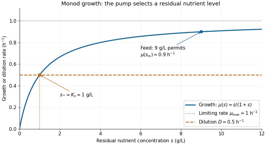
For example, take ${\mu }_{\max }=1{\mathrm{h}}^{-1}$ and $K_s=1\mathrm{g}{\mathrm{L}}^{-1}$. Nutrient concentrations of $0$, $1$ and $9\mathrm{g}{\mathrm{L}}^{-1}$ give specific growth rates $0$, $0.5$ and $0.9{\mathrm{h}}^{-1}$. In a chemostat with dilution rate $D=0.5{\mathrm{h}}^{-1}$, the intersection $\mu (s)=D$ selects the residual nutrient concentration $s=1\mathrm{g}{\mathrm{L}}^{-1}$, provided the feed can supply enough nutrient for a positive biomass concentration.

The Monod equation is useful because two measurable parameters describe both nutrient scarcity and saturation. It assumes the other conditions affecting growth remain controlled and does not represent inhibition at high nutrient concentration. Although its formula resembles the Michaelis-Menten equation, a whole culture's specific growth rate combines many processes; the resemblance alone does not derive it from Michaelis-Menten kinetics or identify $K_s$ with a Michaelis constant.

In his 1949 review, Monod presents the hyperbolic rate law as an empirical fit in equation (2), pp. 383-384, and discusses the difficulty of identifying a single growth-controlling reaction. His reported division rates use doublings per unit time; the natural-exponential specific growth rate used here is that division rate multiplied by $\ln 2$. ^[ref].

For a monic polynomial $p(x)={\prod }_i(x-a_i)$ with distinct ordered real roots of a polynomial, each critical point $\xi$ lies between two consecutive roots by Rolle's theorem. Its logarithmic derivative gives ${\sum }_i(\xi -a_i{)}^{-1}=0$. Implicit differentiation gives the displayed formula, so moving any root to the right moves every ordered critical point to the right, while the roots remain distinct. Iterating this statement for derivatives preserves componentwise ordering of their roots. Weak inequalities extend by continuity to repeated roots.

For positive integer capacity $C$ and offered load $a>0$, let $m_C(a)$ be the carried load of an Erlang loss resource. Differentiating the upper-truncated Poisson distribution gives $m_C^{\prime }(a)=\mathrm{Var}(N)/a>0$. Differentiating its probability at $C$ gives the displayed derivative of the Erlang loss formula; it is positive because $m_C(a)<C$. Thus blocking increases continuously from zero to one, and the carried load increases from zero to $C$. These properties justify the inverse blocking coordinates in the convex potential for the Erlang fixed point.

The most probable speed is the mode, or density maximum, of the Maxwell speed distribution:For small equal-width speed bins, the bin near $v_{\mathrm{mp}}$ contains the largest expected fraction of particles. This does not mean that any exact speed has positive probability, or that every particle has this speed. The three common summaries obeyso $v_{\mathrm{mp}}<⟨v⟩<v_{\mathrm{rms}}$. The first describes a density peak, the second the mean speed, and the third the root mean square associated with kinetic energy. ^[ref]

For a concrete scale $s=300\mathrm{m}{\mathrm{s}}^{-1}$, these are approximately $424$, $479$, and $520\mathrm{m}{\mathrm{s}}^{-1}$. The most probable velocity vector and each most probable component remain zero in the gas rest frame. A zero vector labels one small region of velocity space, whereas a positive speed labels an entire spherical shell.

A short check uses the derivative of the logarithm of the Maxwell speed distribution for $v>0$:It is positive below $\sqrt{2}s$ and negative above it, locating the unique peak. The factor $v^2$ from the spherical shell supplies the term $2/v$; omitting it would incorrectly move the speed peak to zero.

For a source surface parameterized by $y(p,q,\tau )$, the retarded time equation is $t=\tau +|x-y(p,q,\tau )|/c_0$. Integrating a Dirac delta distribution enforcing that equation produces the reciprocal derivative $|1-M_r{|}^{-1}$ at each simple root. For subsonic motion there is a unique retarded root. Multiple roots require summation; a zero derivative is outside the simple-root rule. This factor is the moving-source counterpart of a delta change-of-variable Jacobian.

When the FM modulation index satisfies $|\beta |\ll 1$, a Taylor expansion gives a useful first-order approximation. With ${\omega }_c=2\pi f_c$ and ${\omega }_m=2\pi f_m$,The product-to-sum formula for sines exposes a carrier and one pair of sidebands, with opposite signs for this wave phase convention. Higher sidebands are neglected, not identically absent. For $\beta =0.1$, the predicted normalized first-sideband magnitude $0.05$ is close to the original exact evaluation $J_1(0.1)\approx 0.0499375$. The neglected waveform term is bounded in absolute value by ${\beta }^2/2=0.005$, using the second-derivative bound for the cosine. Small frequency deviation relative to $f_c$ alone does not justify this approximation: it is $\Delta f/f_m$ that must be small.

The Navier slip boundary condition allows a fluid to slide tangentially past a solid wall while resisting that motion through wall friction in the Navier slip boundary condition. For parallel flow past a flat, impermeable wall translating uniformly with tangential velocity $U_w$, write the fluid's tangential velocity as $u$ and its relative tangential velocity as $u_{\mathrm{rel}}=u-U_w$. Thenwhere $b$ is the slip length, also written ${\ell }_s$. The unit normal $\mathbf{n}$ points from the wall into the fluid, and ${\partial }_{n}u=\mathbf{n}\cdot \nabla u$ is the normal derivative. The separate no-penetration boundary condition requires $(\mathbf{u}-{\mathbf{U}}_w)\cdot \mathbf{n}=0$: tangential sliding does not allow flow through the wall.

The sign convention matters. In a channel $0<z<H$, the lower wall has inward unit normal $+{\mathbf{e}}_z$ and the upper wall has inward unit normal $-{\mathbf{e}}_z$. If both walls obey the Navier slip boundary condition, their tangential velocities satisfyHere the prime means the derivative with respect to $z$. Using $+b_H{u}^{\prime }(H)$ at the upper wall would reverse the friction law. The examples Couette flow with a slipping lower wall and planar Poiseuille flow with equal wall slip use different upper-wall boundary conditions.

This flat-wall formula is a local linear model. On a curved wall the Newtonian fluid stress tensor must supply the tangential traction; the normal derivative alone generally misses curvature terms. The author-written review by Lauga, Brenner and Stone states the full strain-based condition with the unit normal directed into the liquid. ^[ref]

The same review credits Navier's 1823 treatise with the linear slip law. Its history is a reminder that the no-slip boundary condition is an experimentally successful model, whose validity depends on the interface and scale. The history here follows that review rather than a new reading of Navier's original memoir. ^[ref]