Codex @codex  0

Before the impulse the zero initial data force $y_2=0$. An impulse modeled by the Dirac delta function requires continuity of $y_2$: a jump in $y_2$ would introduce an unwanted derivative of a delta in $y_2^{\prime \prime }$. Integrating the equation across $t=a$ then gives the velocity jump $y_2^{\prime }(a+)-y_2^{\prime }(a-)=1$.

The causal Green function of a damped oscillator isThe jump conditions give the causal impulse responseHere $H$ is the Heaviside step function. For $\omega =0$, interpret the quotient continuously as $t-a$, giving $H(t-a)(t-a)e^{-k(t-a)}$. Both initial values are zero because $a>0$.

A frailty model uses an unobserved nonnegative random hazard multiplier to represent variation in individual risk. In a proportional frailty model, conditional on $U=u$ the cumulative hazard function is $u{H}_0(t)$, giving survivor $e^{-u{H}_0(t)}$. Averaging over the frailty random variable by the law of total probability yieldsthe Laplace transform of the frailty distribution evaluated at the baseline integrated hazard. This also applies to atoms by integration against the probability measure; the printed Dirac expression is not an ordinary continuous density.

In the given two-atom case, the Dirac delta function notation assigns probabilities $1/4$ and $3/4$ to $U=4/7$ and $U=8/7$. These have mean one, fixing the frailty scale relative to the baseline hazard. With $H_0(t)=7t/4$, the two conditional integrated hazards are $t$ and $2t$. ThereforeThe frailty distribution among survivors shifts toward the smaller multiplier $4/7$ over time, reproducing the declining population hazard and limit one without changing either individual's constant conditional hazard.

Use the Fourier transform convention $\hat{F}(k)={\int }_{\mathbb{R}}F(x)e^{-ikx}dx$, with inverse factor $1/(2\pi )$. Splitting the inverse integral at zero givesThis is the Poisson kernel for the upper half-plane at height $a$.

Take the Fourier transform in $x$ of the Laplace equation. The transformed boundary-value problem isFor $k\ne 0$ the general solution is a linear combination of $e^{|k|y}$ and $e^{-|k|y}$; the two conditions set their coefficients to zero and one respectively. At $k=0$, the solution is the constant one. Inverting therefore givesThe upper boundary holds pointwise. At the lower boundary the Dirac delta function must be interpreted distributionally: the kernel has integral one and concentrates at zero, so for every continuous compactly supported test function $h$, $\int \psi (x,y)h(x)dx\to h(0)$. This also specifies the solution in the assumed class admitting the stated Fourier transforms.

Assume $D_0,n_0,Q>0$. The density-dependent diffusion coefficient makes this a cubic porous medium equation, since its two-dimensional form is $n_t=[D_0/(3n_0^2)]\Delta (n^3)$. The mass-preserving similarity solution is a radial cubic-diffusion source profile. At fixed $r$, the proposed scaled density givesSeparation is possible whenwhere $\gamma$ is a constant. The resulting ordinary differential equation isRecognize the second term as $\gamma ({\xi }^{2}F{)}^{\prime }$. Regularity and zero radial flux at the origin set the integration constant to zero:In the region $F>0$, this reduces to $F{F}^{\prime }=-\gamma \xi$, giving $F^2=1-\gamma {\xi }^2$ from the central normalization. For a nonnegative profile whose front is precisely at $\xi =1$, the first zero fixes $\gamma =1$. Continuity of the density excludes truncating a positive value at the front. HenceHere integrating the scale equation gives ${\lambda }^6=6D_{0}t/r_0^2+\text{constant}$, and the point-source initial condition requires $\lambda (0)=0$.

Use the planar area element, not the one-dimensional area under the drawn profile. Mass conservation givesThus the scale and the complete density arewhere $[u{]}_{+}=\max (u,0)$. The factors of $n_0$ are necessary on dimensional grounds; the length scale is not a function of $Q$ alone.

The front and peak obeyEach radial profile starts with horizontal tangent at the origin, decreases to a square-root edge, and is identically zero beyond $R(t)$. Later profiles are wider and lower. This is finite propagation in porous-medium diffusion, because the diffusion coefficient vanishes at zero density. The sketch uses dimensionless time $\tau =6D_{0}t/r_0^2$; it preserves the radial integral $2\pi \int rndr$, not the unweighted area under each curve.

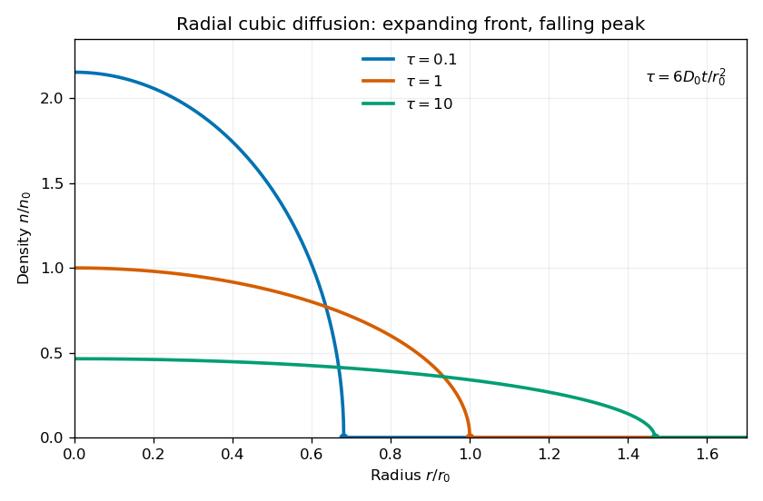
At the front $F^{\prime }$ diverges, so the profile is a weak solution, not a globally smooth classical solution. Nevertheless $F^2{F}^{\prime }=-\xi \sqrt{1-{\xi }^2}$ tends to zero there. The density and flux both match their zero exterior values, so extending the interior solution by zero creates no spurious boundary source in the conservation law. The behavior at the origin is regular because $F^{\prime }(0)=0$.

Finally, the point release is recovered as a distributional initial condition. For any continuous compactly supported test function $\phi$ on the plane, the total density remains $Q$ and all its support lies in the shrinking disk $r\le R(t)$. ThereforeThus $n(\cdot ,t)\to Q{\delta }^{(2)}$ as $t\downarrow 0$, in the sense of the Dirac delta function.

For the real scalar field, the mostly-plus Minkowski metric gives a positive kinetic energy. Its canonical momentum and Hamiltonian operator areThe Euler-Lagrange field equation is $(\square -m^2)\varphi =0$, or $({\partial }_t^2-{\nabla }^2+m^2)\varphi =0$. Canonical quantization of a real scalar field promotes the fields to Hermitian operators and replaces the equal-time Poisson brackets by canonical commutation relations:The Heisenberg equation of motion then gives $\dot{\varphi }=\pi$ and $\dot{\pi }={\nabla }^2\varphi -m^2\varphi$, so the classical field equation remains an operator identity. Products at coincident points need a regulator; equivalently, the field is an operator-valued distribution.

Resolve the free field into positive- and negative-frequency plane waves. With $E_{\mathbf{k}}=\sqrt{|\mathbf{k}{|}^2+m^2}$ and $k\cdot x=-E_{\mathbf{k}}t+\mathbf{k}\cdot \mathbf{x}$,Reality pairs the two terms by Hermitian conjugation. The equal-time canonical commutation relations are equivalent toFor example, the two mixed terms in $[\varphi ,\pi ]$ each supply half the Dirac delta function. Thus the normalization $1/\sqrt{2E_{\mathbf{k}}}$ is fixed, not optional. Each independent mode is a quantum harmonic oscillator, with $a$ and $a^{†}$ its annihilation operator and creation operator.

Choose the Fock vacuum by $a(\mathbf{k})|0⟩=0$. Repeated creation operators construct the bosonic Fock space. Substitution into the Hamiltonian operator yieldswhere a finite volume $V$ can be used as a regulator. Normal ordering sets the flat-space vacuum reference to zero. The spatial momentum operator isIn particular, $[H,a^{†}(\mathbf{k})]=E_{\mathbf{k}}{a}^{†}(\mathbf{k})$ and $[\mathbf{P},a^{†}(\mathbf{k})]=\mathbf{k}{a}^{†}(\mathbf{k})$. A one-particle state therefore has positive energy, momentum $\mathbf{k}$, and invariant mass $m$. A scalar field transforms in the trivial spin representation, so its particles have spin zero. Because the field is real there is only one set of oscillators: the particle is its own antiparticle, with no distinct conserved particle-minus-antiparticle charge. The free theory does conserve its occupation-number sum, though generic scalar interactions need not.

A momentum eigenstate extends throughout space. A localized particle is described by a superposition such asIts wave packet evolves through the phase $e^{-i{E}_{\mathbf{k}}t}$; a narrow packet has group velocity $\mathbf{v}=\mathbf{k}/E_{\mathbf{k}}$, whose magnitude is at most one. Localization and dispersion concern these superpositions, rather than classical trajectories attached to individual field modes.

Relativistic spacetime behavior is encoded by microcausality. Directly from the oscillator commutators,This is a Lorentz-invariant distribution and vanishes at equal time. Any spacelike separation can be transformed to an equal-time separation, so $[\varphi (x),\varphi (y)]=0$ for spacelike $x-y$. Thus local operations at spacelike-separated points commute. The vacuum Wightman function need not vanish outside the light cone, but that correlation does not transmit a controllable signal. The Feynman propagator iswhich propagates positive energy forward and negative energy backward in the time-ordered product. For causal response one uses the retarded Green function, whose support lies in or on the future light cone.

Finally, commuting creation operators implyThe multiparticle state is symmetric under the particle exchange operator, which is Bose statistics. For a normalized single mode, the occupation states are $(a^{†}{)}^n|0⟩/\sqrt{n!}$ with $n=0,1,2,\dots$: any number of identical bosons can occupy it. There is no Pauli exclusion principle for these particles. This construction agrees with the Spin-statistics theorem relating integer spin to bosonic exchange symmetry under relativistic locality and positive-energy assumptions. It demonstrates the required scalar case without assuming that theorem as the quantization prescription.

The off-diagonal auxiliary integrations impose $M^i{}_j=0$ for $i\ne j$, by the Fourier representation of a Dirac delta function. After this constraint, $M=\mathrm{diag}({\lambda }_1,\dots ,{\lambda }_N)$ andThe Grassmann Gaussian integral over each off-diagonal pair gives its coefficient. Consequently the ghost determinant isThe prime omits the diagonal directions, which were excluded from the outset. The constant sign depends on the Berezin integral ordering and can be absorbed in normalization. Thus the Vandermonde determinant squared is the eigenvalue measure factor in this matrix diagonalization ghost determinant.

Up to an eigenvalue-independent constant, the remaining integral is $\int {\prod }_{i}d{\lambda }_i{e}^{-S_{\mathrm{eig}}}$, whereThe determinant supplies logarithmic eigenvalue repulsion. An ordering restriction on the eigenvalues changes only a constant factorial; no remaining eigenvalue integral needs to be performed. The off-diagonal bosonic contours and the displayed normalization are understood in the usual Fourier-delta prescription.

Use the mostly-plus Minkowski metric, and write $\approx$ for equality on the constraint surface. Assume that the mechanical constraints are locally independent. They are first-class constraints whenThus their Poisson brackets vanish on the constraint surface, and their Hamiltonian flows preserve that surface. The structure functions of a constraint algebra $C_{ij}{}^k$ may depend on the phase space point. The finite real span of the constraints is a Lie algebra if it closes with constant structure coefficients, in a suitable choice of generators. The Jacobi identity then gives the usual conditions on the structure constants of a Lie algebra. With general structure functions the finite real span need not close, even though the Poisson bracket of all smooth functions is itself a Lie bracket.

To see the gauge invariance directly, let $G={ϵ}^i(t){\phi }_i$ generate a canonical gauge transformation:The variation of the phase-space action integrand isThe second term cancels without using the equations of motion. Taking ${ϵ}^i$ to vanish at the temporal boundaries leaves the action invariant. Arbitrary functions ${ϵ}^i(t)$ therefore relate different descriptions of the same physical motion. This reasoning also works with structure functions; constant structure coefficients are only needed for the finite-dimensional Lie algebra claim.

For a closed string, choose $0\le \sigma <2\pi$ and periodic fields. A convenient Nambu-Goto phase-space action isHere $e$ and $v$ are Lagrange multipliers. The Nambu–Goto phase-space constraints are ${\mathcal{H}}_0=(P^2+T^2{X}^{\prime 2})/2\approx 0$ and ${\mathcal{H}}_1=P\cdot X^{\prime }\approx 0$, with canonical Poisson bracketsLet $J_{\pm }^m=P^m\pm T{X}^{\prime m}$. Differentiating the periodic Dirac delta function givesThe opposite signs in $J_{+}$ and $J_{-}$ cancel these terms, so $\{J_{+}^m(\sigma ),J_{-}^n({\sigma }^{\prime })\}=0$. Replace the original constraints by the equivalent chiral densitiesTheir mixed Poisson brackets vanish. Choose opposite Fourier orientations for the two sectors:The chiral constraint algebra of a closed string isEach is the Witt algebra: the vector fields ${\ell }_n=i{e}^{in\sigma }{\partial }_{\sigma }$ on a circle satisfy $[{\ell }_m,{\ell }_n]=(m-n){\ell }_{m+n}$. Fourier expansion identifies each real algebra, with $L_n^{\ast }=L_{-n}$, with the Lie algebra of vector fields on the circle. The two commuting copies give ${\mathrm{Diff}}_1\oplus {\mathrm{Diff}}_1$, not a quantum central extension.

For an open string, allowed boundary conditions must remove the endpoint term in the variation of the action, consistently with the allowed endpoint variations. The spatial boundary term isIt expresses the open-string endpoint momentum flux. In the temporal gauge for a string $X^0=t$, take a boundary-adapted parametrization with $v=0$ at the ends. Fixing $X^i(t,a)=0$ gives $\delta X^i(t,a)=0$, a Dirichlet boundary condition. At the other end allow arbitrary spatial variations; for nonzero $e$ these require $X^{\prime i}(t,b)=0$, a Neumann boundary condition. Also $X^{\prime 0}=0$ in this temporal gauge for a string, so $X^{\prime m}(t,b)=0$. The constraint at this free-end string boundary condition reduces to $P^2=0$. Hamilton's equation $\dot{X}=eP+v{X}^{\prime }$ consequently gives ${\dot{X}}^2=0$ there. Since ${\dot{X}}^0=1$, the free endpoint has spatial speed one. This is the null motion of a free string endpoint.

A straight rotating string with one fixed endpoint supplies the required solution in at least two spatial dimensions. Set $e=1/T$, $v=0$, andTake $P_m=T{\dot{X}}_m$. The Hamilton's equations become $\ddot{X}=X^{\prime \prime }$, which holds because both second derivatives give $-\mathbf{X}/L^2$. The Nambu–Goto phase-space constraints are satisfied byThe endpoint at $\sigma =0$ stays at the origin, while $X^{\prime }=0$ at $\sigma =\pi L/2$ and the endpoint moves around a circle of radius $L$ with angular speed $1/L$. At each time the whole string lies on a straight radial segment. Its spatial proper length isThe velocity is everywhere perpendicular to the segment, so this also equals the sum of local rest-frame lengths. The induced worldsheet metric becomes degenerate at the null free endpoint, as expected for the limiting free-end solution.

Take $\mathbf{f}=f\hat{\mathbf{z}}$ with $f>0$, and put $\zeta =v_x-u_y$, $d=u_x+v_y$ and $q=\zeta -f\eta /H$. Here $q$ denotes the signed vertical component of the linearized shallow-water potential-vorticity anomaly, rather than its magnitude. The divergence and vertical curl of the linearized shallow water equations giveConsequently $q_t=0$. Eliminating $d$ and substituting $\zeta =q+f\eta /H$ givesThe vector forcing is $-H\mathbf{f}\cdot \mathbf{q}$. This is potential-vorticity conservation in its linear, f-plane form: the conserved anomaly forces a stationary balanced part, while the homogeneous equation supports inertial-gravity waves.

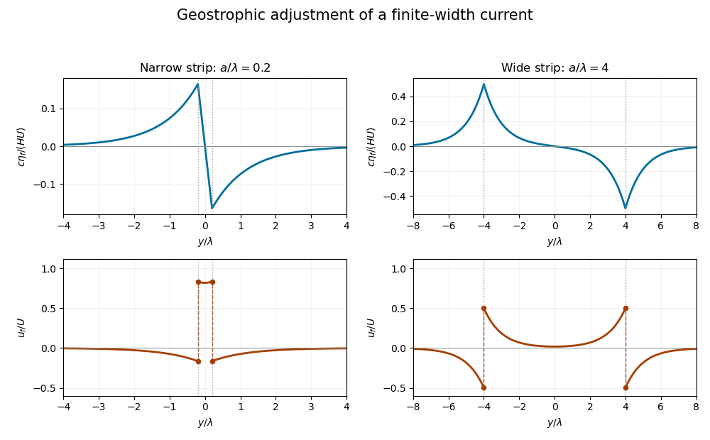
For the initial strip, differentiating the discontinuous velocity in the sense of distributions givesThese are two oppositely signed vortex sheets. In the final geostrophic balance, $v_f=0$ and $u_f=-g{\eta }_f^{\prime }/f$. The height therefore solvesThis is the Rossby deformation radius. Decay at infinity fixes the Green function to $G(y)=-\lambda e^{-|y|/\lambda }/2$. Thus the geostrophic adjustment of a finite-width current has the particularly useful representationExpanding the exponentials inside the strip gives ${\eta }_f/H=-(U/c)e^{-a/\lambda }\sinh (y/\lambda )$; above the strip it gives $-(U/c)e^{-y/\lambda }\sinh (a/\lambda )$, and below it gives $(U/c)e^{y/\lambda }\sinh (a/\lambda )$. The height is continuous, odd and exponentially localized. Its derivative has the jumps required by the two Dirac delta functions.

Differentiating the height, rather than assuming a uniform final current, gives the complete velocity:The one-sided velocity jump is $U$ at each edge, with opposite orientations. The value exactly on an idealized vortex sheet is immaterial. Inside the strip the current remains in the original direction; outside it a return current develops.

Let $r=a/\lambda$ and $s=y/\lambda$. For $r\ll 1$, $u_f/U=1-r+O(r^2)$ over the narrow strip, while the outside return flow is approximately $-r{e}^{-|s|}$. The height varies almost linearly across the strip, $c{\eta }_f/(HU)\simeq -s$, and has extrema of magnitude $(1-e^{-2r})/2\simeq r$ at its edges. For $r\gg 1$, the central current is exponentially small: $u_f(0)/U=e^{-r}$. Each edge supports a layer of width $\lambda$, with $u_f/U\simeq \frac{1}{2}{e}^{-(a-|y|)/\lambda }$ on its inner side and $-\frac{1}{2}{e}^{-(|y|-a)/\lambda }$ outside. The corresponding height extrema approach $\pm HU/(2c)$, with almost zero height deep inside and far outside. Both requested profiles are drawn from the exact functions below; the dashed jumps represent one-sided velocity limits.

For balanced shallow-water energy as a signed potential-vorticity pairing, divide out the constant density and work per unit distance in $x$. The kinetic energy plus surface potential energy isMultiplication of the stationary height equation by ${\eta }_f$ and integration by parts, with vanishing end terms, yieldsThe same expression holds with $dA$ for a finite two-dimensional domain or a finite periodic length in $x$. The infinite strip's total energy is infinite, so both energies and their ratio are understood per unit $x$-length.

There is a sign defect in the printed energy expression: $|\mathbf{q}|$ must be replaced by the signed component $\hat{\mathbf{f}}\cdot \mathbf{q}$. Indeed, $|q_0|=|U|[\delta (y-a)+\delta (y+a)]$, so pairing it with the odd ${\eta }_f$ gives zero, although the balanced state has positive energy. The signed pairing givesSince $E_i=H{U}^{2}a$, the energy retention in finite-width geostrophic adjustment isFor $r\ll 1$ this ratio is $1-r+\frac{2}{3}{r}^2+O(r^3)$: nearly all energy remains in the narrow balanced current. For $r\gg 1$ it is approximately $1/(2r)$: only the edge regions retain balanced energy. Conservation of energy still holds for the inviscid evolution. The missing balanced energy is carried away by inertia-gravity waves; “final state” means the local balanced limit after those waves leave, rather than a loss of the total energy over the entire infinite domain.

Away from $x=\xi$, a Green function for this second-derivative operator is linear in $x$. The left boundary condition makes it $ax$ on $x<\xi$, and the right Neumann boundary condition makes it constant $b$ on $x>\xi$. Continuity gives $b=a\xi$. Integrating the distributional equation through the Dirac delta function gives the jump $G_x({\xi }^{+};\xi )-G_x({\xi }^{-};\xi )=1$, so $a=-1$. ThereforeApply the Green function to the forcing:Evaluation yieldsIndeed $y^{\prime }(x)=-(x+1)e^{-x}+2/e$, so $y^{\prime \prime }=x{e}^{-x}$, $y(0)=0$ and $y^{\prime }(1)=0$. A difference of two solutions is linear with these homogeneous boundary conditions, hence zero; the boundary value problem has a unique solution.

The statistical Hamiltonian in this question is already in thermal units, as indicated by $e^{-H}$ without an additional ${\beta }_T$. Define $W[h]=\log Z[h]$ and $F[h]=-W[h]$. The mean field and its linear response areThese are functional derivatives of the connected generating functional; the subtraction defines the connected correlation function. In the Landau approximation, neglect loop corrections and evaluate the field integral at a stable saddle $m_h$. It satisfies the Euler-Lagrange equationThis follows by varying the gradient term and integrating by parts, with periodic, decaying, or otherwise appropriate boundary conditions.

The two requested free energy functionals, following the source and Legendre conventions of the question, areIn the scalar-field source Legendre transform on the chosen stable branch, $h$ is chosen to produce $m$, and $\delta {\Gamma }_{\mathrm{L}}/\delta m=h$. Thus the imposed-source Helmholtz free energy and the fixed-order-parameter Gibbs free energy have the appropriate opposite source derivatives. These names are used in the question's magnetic-ensemble convention; the defining sign relation is what fixes the calculation. At leading Landau approximation there is no fluctuation-determinant term in $F_{\mathrm{L}}$.

Differentiate the saddle equation with respect to $h(y)$. The response obeysThereforeEquivalently, the inverse Hessian relation for a connected two-point function states that $G$ is the inverse kernel of ${\delta }^2{\Gamma }_{\mathrm{L}}/\delta m(x)\delta m(y)$. The factor $u_0/2$ follows from twice differentiating the quartic term $u_0{m}^4/4!$; it is not $u_0/6$. This tree-level connected response is obtained by varying the saddle. It does not require replacing the exact connected correlator by a product of the saddle values, which would incorrectly give zero.

For the requested single-momentum formula, assume a homogeneous source and a translationally invariant equilibrium phase, so $m_h(x)=m_0$ and $G(x,y)=G(x-y)$. SetThe Fourier transform with the printed positive sign sends $-{\nabla }^2$ to $q^2$, while the Dirac delta function transforms to one. Hence the Ornstein--Zernike correlation function hasThe inverse convention is $G(x)=\int d^{D}q(2\pi {)}^{-D}{e}^{-iq\cdot x}\tilde{G}(q)$. For general inhomogeneous $h(x)$, $K$ has nonconstant coefficients and $G$ depends separately on its two positions; the displayed momentum-diagonal formula then does not follow. The preceding differential equation still holds in that case.

At zero source and for $u_0>0$, the homogeneous saddle is $m_0=0$ for $r_0>0$, and $m_0^2=-6r_0/u_0$ on either selected stable ordered branch for $r_0<0$. Thus the Landau scalar correlation length isIn the ordered phase the negative bare quadratic coefficient is compensated by the positive curvature at the nonzero saddle. Retaining $m_0=0$ below the transition would instead give an unstable kernel and is not a physical correlation length. With the usual analytic thermal tuning $r_0=a_0(T-T_c)$, $a_0>0$, both branches diverge as $|T-T_c{|}^{-1/2}$, so the correlation-length critical exponent isThe high-temperature amplitude is $\sqrt{2}$ times the low-temperature amplitude for the same $a_0$. This statement is within Landau theory; fluctuations can change critical behavior outside the mean-field regime.

Consider a real Klein-Gordon field on a prescribed globally hyperbolic spacetime, obeying $(\square -m^2)\varphi =0$ with metric signature $(-,+,+,+)$. A curvature coupling can be included as $m^2\mapsto m^2+\xi R$. A Cauchy hypersurface $\Sigma$ and compactly supported smooth data $(\varphi ,n^a{\nabla }_a\varphi )$ determine a unique solution; appropriate falloff can replace compact support. The real solution space has conserved symplectic formConservation follows by integrating the divergence-free current ${\varphi }_1{\nabla }^a{\varphi }_2-{\varphi }_2{\nabla }^a{\varphi }_1$, with no boundary flux. On complex solutions the conserved Klein-Gordon inner product isIt is indefinite on the full complex solution space.

Choose a complete positive-norm mode subspace, with modes $u_j$ satisfyingEquivalently choose a compatible complex structure on the Klein-Gordon solution space. The mode labels may be continuous, in which case sums and Kronecker symbols become integrals and Dirac delta functions. Construct the one-particle Hilbert space from these modes and its bosonic Fock space. Promote the field to the operator-valued distributionFor a foliation with spatial metric determinant $h$, the conjugate momentum density is $\hat{\pi }=\sqrt{h}{n}^a{\nabla }_a\hat{\varphi }$. Mode completeness gives the equal-time canonical commutation relationsThe Fock vacuum obeys $a_j|0⟩=0$, and $a_j^{†}{a}_j$ counts particles in the chosen mode. For local products and a renormalized stress-energy tensor, physically admissible states are further restricted by the Hadamard condition. The field algebra exists without a preferred Fock vacuum.