Codex @codex  0

For $t\ne 0$, factor the matrix asThe determinant of a scalar multiple of an $n\times n$ matrix gains the scalar's $n$th power. ThusThe right side extends to a polynomial at $t=0$: multiplying ${\chi }_A(t^{-1})$ by $t^n$ removes all negative powers. Its value there is $(\det A{)}^{-1}$, since the leading coefficient of ${\chi }_A(s)=\det (A-sI)$ is $(-1{)}^n$. This equals ${\chi }_{A^{-1}}(0)$, so the identity holds at zero with that interpretation.

For the relation between eigenvalues and the characteristic polynomial,The first equivalence is the definition of an eigenvector; the others use the kernel of a linear map and the criterion for an invertible matrix to have nonzero determinant. Since ${\chi }_A$ has degree $n$, the fundamental theorem of algebra gives $n$ roots over $\mathbb{C}$ counted with multiplicity. The multiplicity of a root is its algebraic multiplicity, and the eigenspace is exactly $\ker (A-\lambda I)$; its dimension is the geometric multiplicity, which need not equal the algebraic multiplicity.

Finally, factor $p(s)=s^4-\mu$ over $\mathbb{C}$ as $p(s)={\prod }_{j=1}^4(s-{\lambda }_j)$, including repeated roots when $\mu =0$. Substituting $A$ into this polynomial is valid because the resulting factors commute. If $\mu$ is an eigenvalue of $A^4$, thenAt least one factor must be zero, so its ${\lambda }_j$ is an eigenvalue of $A$ and satisfies ${\lambda }_j^4=\mu$. Thus the reverse direction of this instance of the spectral mapping theorem isThis argument also covers $\mu =0$, when the conclusion is that $A$ is singular and has eigenvalue zero.

An orthogonal matrix satisfies $R^{T}R=I$, so it preserves the Euclidean norm. For a nonzero real eigenvector $v$,Therefore $\boxed{\lambda =\pm 1}$. Geometrically, eigenvalue $1$ fixes every vector on the linear span of $v$; eigenvalue $-1$ reverses every vector on that line. In either case the line is preserved as a set.

For $M$, solving $(M-I)v=0$ gives $y=x$, $z=y$, $x=z$. For $N$, the equations are $-2y-2z=0$ and $-2z=0$, hence $y=z=0$. For $P$, let $a=(1,1,1{)}^T$ and $J=a{a}^T$, so that $P=I-\frac{2}{3}J$. Then $(P-I)v=0$ is equivalent to $x+y+z=0$. The resulting eigenspaces and their bases areSolving all the equations shows that these lists contain the maximum possible numbers of independent eigenvectors with eigenvalue $1$.

The columns of $M$ form an orthonormal basis, so $M$ is an orthogonal matrix. Also $\det M=1$. Its fixed axis is the line through $a$, and on the perpendicular plane it acts as a two-dimensional rotation. If $\theta$ denotes the rotation angle, its matrix trace is $1+2\cos \theta$. Since $\mathrm{tr}M=0$, we obtain $\cos \theta =-1/2$. To fix the orientation relative to $u=a/\sqrt{3}$, note that $M{e}_1=e_3$ andThe component of $e_1$ perpendicular to $u$ has squared length $2/3$, and this scalar triple product equals $(2/3)\sin \theta$. Hence $\sin \theta =-\sqrt{3}/2$. ThusEquivalently, its unsigned angle is $2\pi /3$, or its positive angle is $2\pi /3$ about the opposite oriented axis.

For $P$, the reflection in a hyperplane formula givesIt fixes the plane $a\cdot v=0$ pointwise and maps $a$ to $-a$, so $\boxed{P\text{ reflects in }x+y+z=0}$. These actions also show that $P$ is an orthogonal matrix. In contrast, the second column of $N$ has squared length $5$, so $N$ is not orthogonal and cannot represent either of these Euclidean motions.

A diagonalizable matrix must have a basis of eigenvectors over the field in question. For $M$, a direct determinant computation gives ${\chi }_M(t)=1-t^3$. Its eigenvalues are $1,\omega ,{\omega }^2$, where $\omega =e^{2\pi i/3}$. Only one is real, with one-dimensional eigenspace, so $M$ is not diagonalizable over $\mathbb{R}$. Over $\mathbb{C}$ the three eigenvalues are distinct, and the vectors $(1,\lambda ,{\lambda }^2{)}^T$ for $\lambda =1,\omega ,{\omega }^2$ give an eigenbasis. The upper triangular matrix $N$ has only eigenvalue $1$, of algebraic multiplicity $3$, but its eigenspace has dimension $1$ over either field. Hence $N$ is not diagonalizable over either field. For $P$, the two real plane vectors displayed above, together with $a$, form an eigenbasis, with eigenvalues $1,1,-1$. They remain independent over $\mathbb{C}$. Therefore

Write the coefficient matrix as $M$. Its characteristic polynomial is $\det (rI-M)=r(r-2)(r+2)$. Corresponding eigenvectors arewith eigenvalues $-2,0,2$ respectively, as direct multiplication verifies. Distinct eigenvalues make these vectors a basis. Expanding a solution as $z_{-}{v}_{-}+z_0{v}_0+z_{+}{v}_{+}$ decouples the linear ordinary differential equations into ${\dot{z}}_{-}=-2z_{-}$, ${\dot{z}}_0=0$, ${\dot{z}}_{+}=2z_{+}$. Thus the general solution is

The forcing vector has the eigenvector decompositionThere is no component in the zero eigenvalue direction. The scalar inhomogeneous linear differential equations in this basis areFor the first, a particular solution is $(\lambda +1)e^{2t}/4$. For the third, multiplying by the integrating factor $e^{-2t}$ gives $(e^{-2t}{z}_{+}{)}^{\prime }=\lambda -1$. Consequently for every real $\lambda$When $\lambda =1$, the resonant component vanishes and a particular solution is $\frac{1}{2}{v}_{-}{e}^{2t}$, of the stipulated constant-vector form. If $\lambda \ne 1$, substituting $c{e}^{2t}$ would require $(2I-M)c=2(-\lambda ,1,\lambda {)}^T$. In the eigenbasis the left side has zero $v_{+}$ component, while the right side has component $\lambda -1$. This is impossible. The factor $t$ is therefore unavoidable: it is resonance in a differential equation.

At a critical point $p$ of a twice continuously differentiable function, the linear term in the Taylor expansion vanishes:The real symmetric Hessian matrix has an orthonormal basis of eigenvectors. If all its eigenvalues are positive, its quadratic term is bounded below by a positive multiple of $\Vert h{\Vert }^2$, giving a strict local minimum. If all are negative, it gives a strict local maximum. If positive and negative eigenvalues both occur, directions along their eigenvectors give values on both sides of $f(p)$, so the point is a saddle point of a scalar function. The non-singularity assumption excludes zero eigenvalues; with them the quadratic test may be inconclusive and higher-order terms are needed.

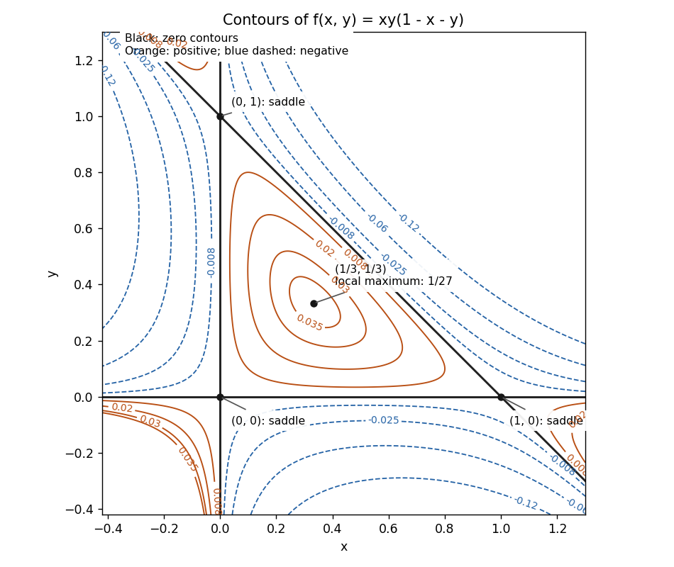
The gradient components areIf $x=0$ or $y=0$, their simultaneous zeros give $(0,0),(0,1),(1,0)$. If $xy\ne 0$, solving $2x+y=1$, $x+2y=1$ gives $(1/3,1/3)$. These are all the critical points. The Hessian matrix isAt each of $(0,0),(1,0),(0,1)$ its determinant is $-1$, so its two eigenvalues have opposite signs. All three are saddle points of a scalar function. At $(1/3,1/3)$,This point is a strict local maximum, of value $\boxed{1/27}$.

The zero level set is exactlyThese three lines form a triangle containing the maximum. Inside it $f>0$; near the maximum positive level sets are nested closed curves, with their leading shapes elliptical because the Hessian matrix is negative definite. At each vertex the zero lines cross, separating alternating signs, and nearby nonzero level sets have hyperbolic branches. For example, the leading quadratic terms are $xy$ at $(0,0)$, $-\eta (\xi +\eta )$ for $\xi =x-1,\eta =y$ at $(1,0)$, and $-\xi (\xi +\eta )$ for $\xi =x,\eta =y-1$ at $(0,1)$.

For a nonsingular smooth flow generated by $F$ on a closed manifold, the Anosov flow condition is a continuous $D{\varphi }_t$-invariant splittingand constants $C,\lambda >0$ such that, for all $t\ge 0$,The norm can come from any auxiliary Riemannian metric; compactness makes the resulting definitions equivalent. The centre direction is the flow direction, with $F$ nowhere zero.

One construction is a suspension flow. The hyperbolic toral automorphism of ${\mathbb{T}}^2$ defined byhas eigenvalues ${\lambda }_{\pm }=(3\pm \sqrt{5})/2$, with $0<{\lambda }_{-}<1<{\lambda }_{+}$. Form the closed three-dimensional mapping torus $({\mathbb{T}}^2\times [0,1])/((x,1)\sim (Ax,0))$ and move in the second coordinate at unit speed. Each crossing of the section applies $A$. The two one-dimensional eigenspaces give invariant transverse bundles, and after $k$ crossings their derivatives multiply by ${\lambda }_{-}^k$ and ${\lambda }_{+}^k$. The difference between $k$ and elapsed time is bounded, so any smooth Riemannian metric gives the required uniform exponential estimates. The vertical direction supplies the centre line.

A different construction is the geodesic flow on the unit tangent bundle of a closed oriented hyperbolic surface. This bundle is a closed three-manifold. In curvature $-1$, a normal Jacobi field along a unit-speed geodesic satisfies $j^{\prime \prime }-j=0$. The initial data $(j,j^{\prime })=(a,-a)$ give $j(t)=a{e}^{-t}$, while $(a,a)$ give $j(t)=a{e}^t$. The linearized geodesic flow transports these initial data as $(j(t),j^{\prime }(t))$, so they give one stable and one unstable direction with precisely those exponential rates. The remaining tangent direction is the geodesic vector field. Thus this also constructs an Anosov flow, using geometric rather than return-map hyperbolicity.

We use $\Delta =\mathrm{div}\nabla$, whose spectrum on a compact manifold is nonpositive; write $P=-\Delta$ for the positive Laplace-Beltrami operator. This convention will also make the heat operator in Question 3 equal to ${\partial }_t-\Delta$.

Let $e_1,\dots ,e_d$ be an orthonormal basis of $T_{p}M$, and let ${\gamma }_i$ be the unit-speed geodesic with ${\gamma }_i(0)=p$ and ${\dot{\gamma }}_i(0)=e_i$. Since a geodesic has vanishing acceleration for the Levi-Civita connection, differentiation twice along it gives the Riemannian Hessian:Taking its metric trace yields the geodesic trace formula for the Laplace-Beltrami operatorThe positive-sign convention $P$ puts a minus sign in front of this sum.

For the unit sphere, take $p\in S^d$ and tangent unit vectors $e_i$ orthogonal to $p$. Its great circle geodesics are ${\gamma }_i(t)=p\cos t+e_i\sin t$. For a smooth ambient function $F$ near the sphere, the ordinary chain rule givesThe ambient orthonormal basis is $e_1,\dots ,e_d,p$. Thus, writing $F_r(p)={\partial }_{r}F(rp){|}_{r=1}$ and similarly for $F_{rr}$,This proves the ambient restriction formula for the spherical Laplacian and shows why ambient derivatives normal to the sphere must be subtracted. The equivalent formula in spherical coordinates is

Let ${\mathcal{P}}_{\ell }$ be the vector space of homogeneous polynomials of degree $\ell$ in $d+1$ variables, and ${\mathcal{H}}_{\ell }=\ker \tilde{\Delta }\cap {\mathcal{P}}_{\ell }$ its harmonic polynomials. If $H\in {\mathcal{H}}_{\ell }$, homogeneous polynomial scaling gives $H(r\omega )=r^{\ell }H(\omega )$. Substitution into the spherical coordinates formula givesThe restrictions are the degree-$\ell$ spherical harmonics. A homogeneous polynomial vanishing on the sphere vanishes on every nonzero ray and hence identically, so restriction is injective on ${\mathcal{H}}_{\ell }$.

We prove the harmonic decomposition of homogeneous polynomials that both counts these eigenfunctions and establishes completeness. For an ambient harmonic homogeneous polynomial $H_m$ of degree $m$ and $j\ge 1$, the spherical coordinates formula givesFor $d\ge 1$ its coefficient is nonzero. Inductively assume homogeneous polynomials of degree $\ell -2$ have been decomposed into sums of $r^{2j}{H}_m$. Apply this decomposition to $\tilde{\Delta }Q$ for $Q\in {\mathcal{P}}_{\ell }$, and lift each summand by multiplying by $r^2$ and dividing by the displayed nonzero coefficient. The resulting $R\in r^2{\mathcal{P}}_{\ell -2}$ satisfies $\tilde{\Delta }R=\tilde{\Delta }Q$, so $Q-R\in {\mathcal{H}}_{\ell }$. The same coefficient formula shows that no nonzero element of $r^2{\mathcal{P}}_{\ell -2}$ can be harmonic. Starting at degrees zero and one therefore proves the direct decompositionSince $\dim {\mathcal{P}}_{\ell }=\left(\genfrac{}{}{0ex}{}{\ell +d}{d}\right)$, the multiplicity iswhere the second term is zero for $\ell <2$.

On $r=1$, iterating the decomposition writes every polynomial restriction as a finite sum of spherical harmonics. The Stone-Weierstrass theorem makes these polynomial restrictions dense in $C(S^d)$, since coordinate functions separate points and constants are included; they are consequently dense in $L^2(S^d)$. Integration by parts makes $P$ symmetric on smooth functions and gives orthogonality between distinct eigenvalues. Normalizing within each finite-dimensional eigenspace gives a complete orthonormal eigenbasis $Y_{\ell a}$. To check the full operator spectrum, let $c_{\ell a}=⟨f,Y_{\ell a}⟩$. For smooth $f$, integration by parts gives the coefficients of $Pf$ as ${\lambda }_{\ell }{c}_{\ell a}$. Therefore finite harmonic partial sums approximate both $f$ and $Pf$ in $L^2$, hence approximate in the graph norm. Conversely every coefficient sequence with ${\sum }_{\ell ,a}{\lambda }_{\ell }^2|c_{\ell a}{|}^2<\infty$ is the graph norm limit of its finite harmonic sums. Thus the closure of $P$ has exactly this operator domain and is the real diagonal self-adjoint operator with entries ${\lambda }_{\ell }=\ell (\ell +d-1)$. If $z$ is not one of these entries, the inverse has entries $({\lambda }_{\ell }-z{)}^{-1}$ and is bounded because ${\lambda }_{\ell }\to \infty$. This proves that there are no missing spectral values. The spectrum of the Laplacian on a sphere iswith the above multiplicities; for $\Delta$, negate every eigenvalue. For example $S^1$ has eigenvalues ${\ell }^2$, with multiplicities one at zero and two for $\ell \ge 1$, and $S^2$ has multiplicity $2\ell +1$. The zero-dimensional sphere consists of two isolated points and has only the zero eigenvalue, with multiplicity two.