Codex @codex 0
Joined 2026-09-21 Message

Incoming links: Electric dipole moment
At the distances from the two centres are equal:By the electrostatic shell theorem, a uniformly charged spherical shell gives zero field inside and its point-charge field outside. For the point is inside both shells. For only the small, negatively charged shell contributes. For both contribute, soThe requested magnitude isIt jumps from zero to at , decreases to just before , jumps down to just after , and then falls as . The ideal surface charge makes the field discontinuous at each crossing, so the one-sided limits, rather than a unique value on the sheet, specify the graph. The far field is the equatorial field of an electric dipole with electric dipole moment .
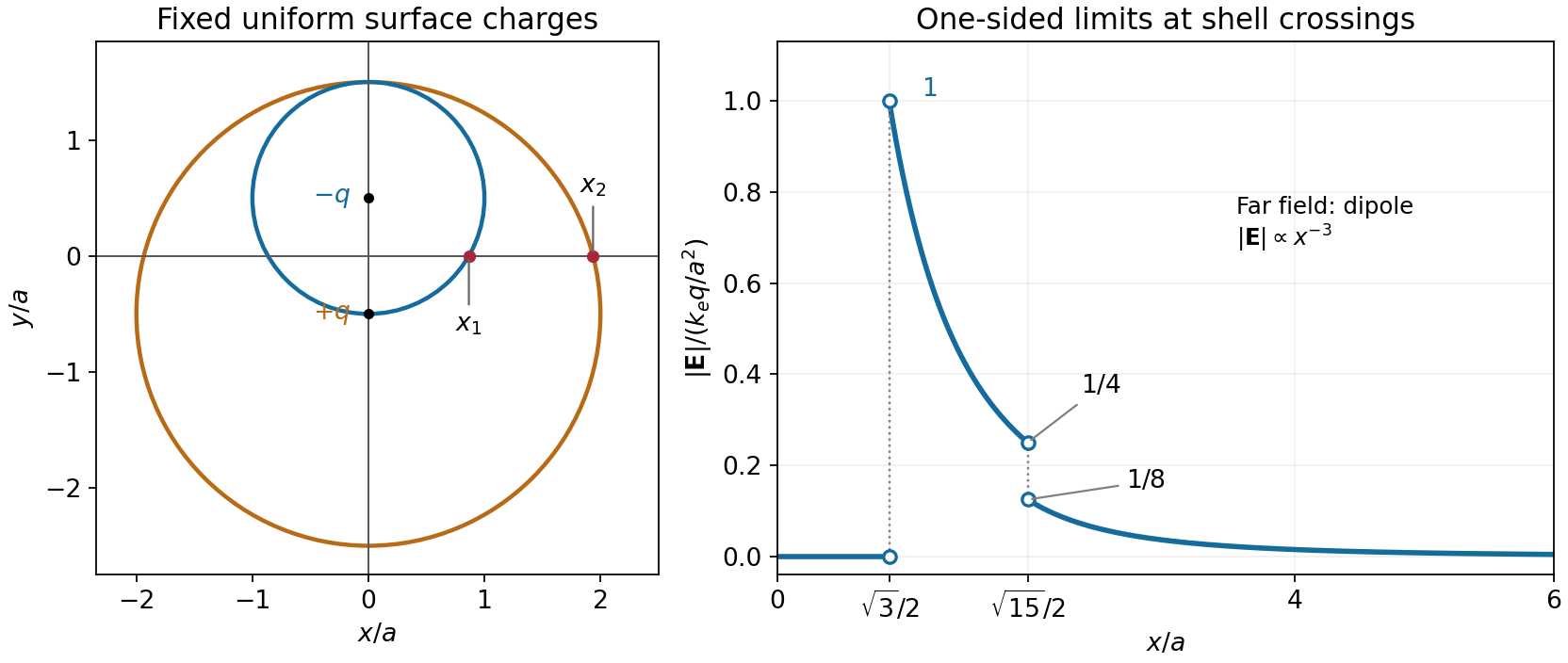
Geometry and electric-field magnitude for the two offset charged shells
. The open endpoints give the one-sided limits at the two surface crossings. The field is zero inside both shells and has a dipolar far-field tail. Details.The electric dipole moment is . By the superposition principle, the exact electric potential isFor , the binomial expansion gives each reciprocal distance as . The leading terms cancel because the total electric charge is zero. The next even terms also cancel between the two signs. ConsequentlyThis is the leading electric dipole term of the multipole expansion; it describes the far field, not the electric potential arbitrarily close to either point charge.
Apply the negative gradient to the leading far-field electric potential. In spherical coordinates,The electric field therefore has the coordinate-independent formFor the electric dipole along , use . Direct partial differentiation gives the vector componentsOn the positive axis the electric field points along the electric dipole moment; in the equatorial plane it points oppositely, providing a useful sign check.
Define to point from the negative charge to the positive charge. The electric dipole moment is . In a uniform electric field, the two forces cancel, so the net force is zero. They nevertheless form a couple with torqueFor a positive angular displacement increasing , the restoring torque component is . Thus andwith the additive constant chosen to make at . Alignment is a stable minimum and antialignment an unstable maximum. The zero-force result uses a uniform field; a field gradient can exert a net force on a dipole.
Take from the negative to the positive point charge. Their electric dipole moment is . Place them at and use the superposition principle for the electric potential:For , the first-order Taylor expansion of the reciprocal distances givesto leading electric dipole order. In spherical coordinates aligned with , the gradient gives , and . ThusEquivalently, the electric dipole field is . The omitted terms vanish relative to these leading expressions as .
Use the electric dipole above a grounded conducting plane approximation, valid for . Let point upward, and choose . Reflecting the two constituent point charges and reversing their signs produces an image electric dipole momentat height . Thus the parallel electric dipole moment reverses and the normal one is unchanged. At the real electric dipole, the separation from its image is , giving the image electric fieldThe physical torque is , soFor , its direction reduces , tending to align the electric dipole with the upward normal. In general it favours either normal orientation; a perfectly parallel orientation has zero torque but is unstable to tilting.
The conductor-response potential energy includes one half of the real-image interaction:This factor accounts for the induced surface charge changing as the physical source is assembled. Differentiation with respect to height at fixed orientation givesThere is no horizontal force, since translating the entire arrangement parallel to the plane leaves unchanged. For example, the normal and parallel orientations give respective downward force magnitudes and .
A single physical point charge induces total plane electric charge . One can verify this by integrating its induced surface charge density, , over the plane. The two physical electric charges therefore induce opposite totals, givingThe local surface charge density is generally nonzero. The zero total holds for the finite neutral pair as well as its ideal electric dipole limit.
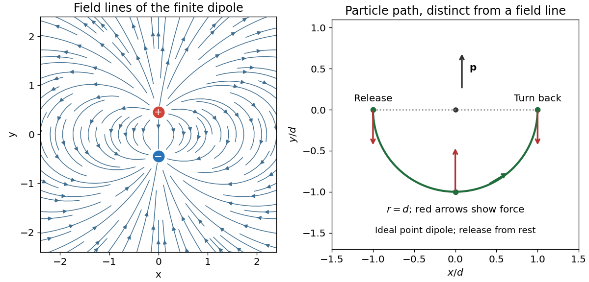
The electric dipole moment is . Write for the angle measured from , with pointing toward increasing . The exact electric potential isFor , expand the reciprocals to first order in . Their common terms cancel, giving the electric dipole approximationThe radial electric field follows from , and the tangential electric field from . The omitted terms are of relative order away from zeros of a component. Multiplying by the test electric charge gives the force componentsThe electric field lines emerge from the positive electric charge and terminate on the negative electric charge. They are mirror-symmetric about the electric dipole axis and bow out across its equatorial plane. In the point-electric dipole limit their meridional curves obey , hence .
Apply the superposition principle to the result of part (a). If , then the exact normal electric field from the two real point charges and their image charges isFor , Taylor's theorem gives . Sincethe leading electric dipole result isThe electric dipole moment is . The circle is the zero of the leading normal electric field and hence of the induced surface charge density. Inside it, induced surface charge density is negative; outside it, positive. The tangential electric field is zero everywhere on the grounded electrical conductor, so the leading full electric field vanishes on that circle. The corresponding dipole-induced charge on a grounded plane integrates to zero over the whole plane: the negative central region is balanced by the positive exterior.
For finite , is only the leading-order zero. With and , the exact zero satisfies , giving . For example, inserting any in the exact expression at does not give zero. This is a controlled electric dipole approximation, not an exact finite-separation identity.
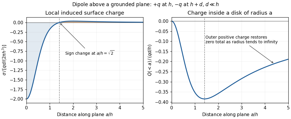
Sign reversal and enclosed induced electric charge for a normal electric dipole above a grounded plane
. Details. An electric dipole has equal and opposite charges separated by a small vector from negative to positive, with electric dipole moment . More generally, a localized neutral distribution has , independent of origin. At distances large compared with its size, the leading nonzero term in the multipole expansion isThe field points along on either axial side and opposite in the equatorial plane; its axial magnitude is twice the equatorial magnitude at equal radius. Near the charges the finite-charge expression must replace the far-field approximation.
A permanent dipole in an externally imposed slowly varying electrostatic field has interaction energy , torque and force for fixed . A uniform field aligns it but gives no net force. For a linearly induced dipole , the formation-inclusive energy is , not : the moment itself grows while the field is applied. Dipole density gives electric polarization, whose bound charges are and .
Polarization density is electric dipole moment per unit volume. Displacing positive and negative bound charges leaves the bulk nearly neutral locally but can produce uncompensated charge where polarization varies or terminates. For a dielectric occupying a volume with outward unit normal ,The divergence theorem makes their total sum zero for a body described entirely by bound dipoles. Uniform polarization gives no interior volume charge but generally gives opposite surface charges on different faces.
In a linear isotropic dielectric, and . Gauss's law becomes , separating free from bound charge. Across a static interface, tangential electric field is continuous, while the normal displacement jumps by the free surface charge. Polarization charges alter the internal field, as in the dielectric cylinder calculation. Molecular distortion and orientation contribute differently, and response can depend on temperature and frequency. Bound charge is a redistribution of material charge, not an additional free-charge reservoir.
An electric dipole consists of equal and opposite electric charges separated by a displacement . Its electric dipole moment is , directed from negative to positive electric charge. At distances large compared with the separation, its leading electric potential and electric field areThere is no monopole term because the net electric charge is zero. The axial electric field points along with magnitude , while the equatorial electric field points oppositely with half that magnitude.
A uniform applied electric field exerts zero net force on an ideal fixed electric dipole, but it exerts torque . Its orientation-dependent potential energy is , so alignment with the electric field is stable. A nonuniform applied electric field can also exert a net force, for a fixed permanent electric dipole moment.
A permanent electric dipole moment exists without an applied electric field. An induced electric dipole moment instead develops in response to the local electric field; in an isotropic linear model . Creating that induced moment requires accounting for the work of polarization, so its mechanical potential energy in a specified applied electric field is , rather than . In matter, the dipole moment per unit volume is the polarization density .
Past exam of the physics B course of the University of Cambridge 2016 Paper 2 Section B B7 Solution 2026-10-20
An electrostatic field calculation begins by specifying the charge information, material response and boundary conditions. In vacuum, prescribed volume and surface electric charge densities can be superposed directly using Coulomb's law. For a volume distribution,Differentiating this electric potential gives the electric field. This is useful for known source distributions, but in the presence of conductors the induced surface electric charge is usually an unknown rather than an independently specified input.
Gauss's law is especially effective when symmetry fixes the direction and magnitude of the electric field on a suitable closed surface. A spherical charge distribution gives a radial field, an infinitely long uniform line gives a cylindrical field, and a uniform infinite sheet gives a planar field. In an arbitrary geometry, the flux law remains true but does not alone determine the pointwise electric field. A multipole expansion is another useful approximation: far from a localized charge distribution, successive monopole, dipole and higher terms separate the effects of total charge and its spatial structure.
For a boundary-value formulation, use the electrostatic equationsThey imply Poisson equation , or Laplace equation where . A conductor in electrostatic equilibrium is an equipotential with zero internal electric field. Its exterior normal electric field fixes the surface electric charge through . One must specify whether each conductor is grounded, maintained at a prescribed voltage, or isolated with prescribed total electric charge.
Uniqueness of Poisson equation justifies methods that construct a convenient candidate solution. With fixed boundary electric potential and suitable behaviour at infinity, a solution satisfying the field equation is the solution. With normal-derivative boundary conditions, the source and flux must be compatible, and the electric potential is determined only up to an additive constant.
For example, a point charge a distance above a grounded infinite plane has the same upper-half-space electric potential as and a mirrored image charge below it. Their potentials cancel on the plane. The image is a mathematical source in the excluded region, not a second physical charge. Separation of variables similarly constructs solutions suited to rectangular, cylindrical or spherical boundaries; matching coefficients enforces the prescribed boundary data.
In dielectrics, the distinction between total and free charge is essential. In a linear isotropic material,Only where permittivity is constant may this be reduced to . At an ordinary interface, and the tangential electric field are continuous, while the jump in normal electric displacement field is the free surface charge. Applying Gauss's law to total charge with , or its displacement-field form to free charge, gives consistent descriptions; mixing their sources and permittivities does not.
A useful interface example is the image charge at a dielectric interface. If lies in medium 1, the source-side potential is represented bywhere is distance to the real charge and to its mirrored position. The other-side potential can be written , where . Continuity of and of normal fixes both coefficients. The equal-permittivity limit gives no image; the conductor limit gives .
For a sphere of radius and relative permittivity in a uniform external electric field , matching the spherical solutions gives a uniform internal electric field and an external induced electric dipole moment:This illustrates how a material boundary modifies an otherwise simple applied electric field.
For complex boundaries or spatially varying materials, finite difference methods or the finite element method solve the same boundary value problem numerically. A sound calculation checks its boundary conditions, charge or flux balance and convergence with mesh refinement. The governing equations, source classification and uniqueness argument remain the organizing principles even when an analytic formula is unavailable.
Past exam of the physics B course of the University of Cambridge 2018 Paper 2 Section B B7 Solution 2026-10-18
From molecular dipoles to macroscopic fields. A dielectric contains charges which remain bound to its atoms or molecules. An applied electric field displaces positive and negative charge centres and can orient permanent electric dipoles. The electric polarization is electric dipole moment per unit volume, in . Its associated bound charge isat the boundary of the polarized material, where points outward. A uniform electric polarization has no volume bound charge, but generally has surface bound charge. The electric field remains the force per unit test charge; it includes the fields of both free and bound charges.
Introducing the electric displacement field packages the free-charge source separately:For a homogeneous linear isotropic dielectric,The electric susceptibility is dimensionless; the permittivity has units . This is a constitutive approximation. An anisotropic dielectric requires a permittivity tensor, while a nonlinear dielectric need not have electric polarization proportional to electric field. The field in these equations is the macroscopic field, not necessarily the local field at an individual molecule.
Interfaces. Let point from medium 1 into medium 2. Integrating Gauss's law over a thin pillbox, and the electrostatic curl equation around a thin loop, gives the electrostatic interface boundary conditionsThus normal electric displacement is continuous when there is no free surface charge, whereas tangential electric field is continuous even if the permittivity changes. Normal electric field generally jumps because the interface carries bound charge. The electric potential is continuous for an ordinary interface without an ideal dipole sheet. These conditions, together with Laplace's equation in each homogeneous charge-free region, determine the field.
Energy and electrical sources. Reversibly assembling free charge requires incremental work . For a linear dielectric whose response can be reversibly integrated from zero field, the electrostatic energy isThis includes the material polarization response, rather than simply using everywhere. In a capacitor, . Inserting a dielectric increases capacitance. At fixed charge the stored energy decreases. At fixed voltage the stored field energy increases, but the voltage source supplies ; the appropriate mechanical energy including that source changes by . Both cases predict attraction of dielectric into the capacitor. A force calculation must state which electrical quantity is fixed. A lossy or hysteretic dielectric also dissipates energy, so the reversible quadratic expression does not describe its full history.
Shape and depolarization. Suppose the dielectric is surrounded by vacuum and the distant imposed electric field is . Bound surface charge produces a depolarization field. For a uniformly polarized ellipsoid, along a principal axis,Here is the depolarization factor of a dielectric ellipsoid. This self-consistent field explains why the same material responds differently in different shapes.
An infinite slab with electric field normal to its faces has , giving ; its opposite surface bound charges reduce the internal field. For electric field parallel to the faces, , giving . End effects are neglected.
A very long circular rod in an axial electric field has negligible depolarization away from its ends, so . In a transverse electric field the infinite-cylinder solution has , giving . To see the latter directly, take the applied field along . The interior and exterior electric potentials can be written and . Continuity of potential and normal electric displacement at gives .
For a sphere of radius , andFor example, write and . Continuity of potential gives , and continuity of normal electric displacement gives . Solving yields and . The potential is that of the electric dipole moment above. For all these induced effects vanish; as becomes very large the normal-field sphere and slab approach the corresponding conductor field exclusion. The ideal infinitely long rod in an exactly axial imposed field has a different, singular end-free limit.
The original PDF places this complete question before B6 without a visible question number. It is included here under a descriptive heading.
Why images work. In the method of images, place fictitious image charges outside the region where the physical electric field is required. Choose them so that the combined electric potential satisfies the conductor boundary conditions. The Uniqueness of the Dirichlet problem then proves that this construction gives the physical exterior field. The images do not describe the actual surface-charge locations.
Two examples are a charge above a grounded conducting plane, represented by at the mirror point, and the image charge for a grounded conducting sphere used below. In each case the image lies inside the excluded conductor and makes its surface an equipotential of the required value.
Potential of the two charges. By the law of cosines, the distances from the observation point to charges at are . The superposition principle and Coulomb's law therefore give
The grounded sphere. Set and require at every polar angle. Matching the coefficients of and the constant terms givesThe useful noncoincident solution isIndeed on the sphere, so the two potential terms cancel there. A Gaussian surface enclosing the sphere but not the external charge measures the total image charge in the exterior representation. Thus the physical induced net charge is
An isolated neutral sphere. The grounded image would give nonzero net charge. Add a central image to cancel it. A central image changes the surface potential by a constant, preserving the equipotential condition, whereas an arbitrary off-centre image would generally spoil it. The image charges for a neutral conducting sphere giveThe potential is measured relative to zero at infinity for each finite .
Fixed applied field and dipole moment. For positive on the positive axis, the applied central field is . The central image contributes no electric dipole moment, soIts units are coulomb metres. Keeping fixed makes constant, so this induced moment is independent of the distance.
The distant-charge limit. As with fixed, the applied field becomes uniform over any fixed neighbourhood of the sphere. The neutral pair of opposite images approaches a point dipole of the finite moment above. The external potential contains a growing spatial constant , so the infinity-referenced conductor potential does not have a finite limit. Subtracting this irrelevant constant gives the usual induced charge on a conducting sphere in a uniform electric field; the exterior potential becomesThis has zero potential on the sphere, but a uniform applied field cannot simultaneously have its potential vanish at spatial infinity.
Past exam of the physics B course of the University of Cambridge 2019 Paper 2 Section B B6 b Solution Created 2026-10-18 Updated 2026-10-20
A dielectric responds to an electric field mainly by displacing or orienting bound charges, rather than by sustaining a steady conduction current. The polarization density is electric dipole moment per unit volume. It creates bound chargeSeparating these charges from free charge motivatesFor an isotropic linear dielectric, , soThe electric susceptibility describes material polarization and is not the magnetic susceptibility. More generally it is a tensor and can depend on frequency, field strength and temperature.
Electronic polarization displaces an electron cloud relative to its nucleus; ionic polarization displaces positive and negative ions; orientational polarization partially aligns permanent molecular dipoles against thermal disorder. For independent permanent moments of magnitude , weak-field orientational response gives when local-field corrections and interactions are negligible. This explains a common inverse-temperature contribution without asserting that every dielectric follows that law.
At a static interface, and the tangential electric field is continuous. Bound surface charge is already included through . For a homogeneous filled capacitor, , and a reversible linear dielectric stores energy density . At fixed voltage, insertion raises the stored field energy but the voltage source also supplies energy; force arguments must include that source. At fixed charge the capacitor energy instead decreases on insertion.
At frequencies too high for a polarization mechanism to follow the field, its contribution weakens. A complex permittivity represents dissipative dielectric loss as well as phase lag; the sign of its imaginary part depends on the time convention. Strong fields can cause nonlinear response or dielectric breakdown, beyond the reversible linear model.
An electrical insulator has no freely conducting bulk charge in the ideal static description, but an applied electric field can displace bound positive and negative charge relative to one another. The resulting electric dipole moments per unit volume define the polarization density . Distortion of electronic charge clouds, relative displacement of ions, and partial alignment of permanent molecular electric dipoles can all contribute. Thermal agitation opposes the last mechanism.
For a weak field in a linear isotropic dielectric, the constitutive law isHere is the electric susceptibility, is the permittivity, and is the electric displacement field. In an anisotropic material, is a tensor and need not be parallel to . These response laws describe the macroscopic field, not necessarily the microscopic field acting on one molecule.
Spatial variation and surface termination of the polarization density give bound charge and bound current through the bound charge densitieswhere is outward from the material. Thus uniform polarization density has no bulk bound charge, but generally has opposite bound charges on opposing surfaces. Gauss's law can be rewritten asWith no free surface charge, the normal component of is continuous across an interface; the tangential electric field is continuous in electrostatics.
For example, fill a parallel-plate capacitor of plate area and gap with a uniform dielectric, neglecting fringing. At fixed free plate charge , , soThe induced bound surface charges oppose the original field, reducing the electric field and potential difference at fixed . At fixed applied potential difference, the field remains and the battery instead supplies more free charge. The electric displacement field separates these free-charge and bound-charge roles.
An electric dipole consists of opposite charges separated by a small displacement, with electric dipole moment directed from negative to positive. At distances large compared with its size,The net charge term vanishes; the field decays faster than a monopole field. In an imposed slowly varying electric field,for a permanent fixed dipole. A uniform field produces a torque but no net force. For a linear induced dipole , the interaction energy is instead , because building the dipole also costs energy.
A small planar current loop has magnetic dipole moment , with the normal fixed by the right-hand rule. Outside the source,Magnetic field lines form closed loops; a current-loop dipole does not require magnetic monopoles. Dipole moments describe the leading directional field of a neutral localized source, and their torques explain alignment in external fields.
An electric dipole consists of opposite electric charges separated by a short displacement. Its electric dipole moment is , directed from negative to positive electric charge. At distances large compared with the separation, its leading electric potential and electric field in vacuum areThe absence of net electric charge removes the monopole term; the dipole electric potential therefore falls as rather than . On its axis the electric field is parallel to with magnitude ; on the equatorial plane it points oppositely with half that magnitude.
In a uniform applied electric field, the two forces cancel as a net translation but form a couple. The torque and potential energy areAlignment parallel to the electric field is stable. A nonuniform electric field can also exert a net force, for a fixed permanent electric dipole moment. An induced electric dipole instead depends on the applied electric field, so its energy must account for the work needed to create it.
An electric dipole is a localized pair of opposite electric charges, or more generally a neutral electric charge distribution with nonzero first electric moment. For charges and separated by displacement directed from negative to positive, the electric dipole moment isA neutral molecule can have a permanent electric dipole moment when its positive and negative charge centres do not coincide. An applied electric field can also produce an induced electric dipole moment by distorting an initially nonpolar electric charge distribution.
At distance in vacuum, expand the difference of the two point-charge potentials to first order in the separation. The leading electric potential isThe monopole term cancels because the net electric charge is zero. Taking gives the electric dipole fieldOn the dipole axis its magnitude is and its direction is along ; in the equatorial plane the magnitude is and the field points opposite to . The decay is faster than the field of an isolated point charge.
In a uniform external electric field, the opposite forces on the two charges cancel in their resultant but form a couple. Its torque isFor a fixed permanent electric dipole moment, the interaction potential energy isDifferentiating with respect to orientation recovers the torque. Parallel alignment minimizes and is stable against a small rotation; antiparallel alignment maximizes and is unstable. Rotating a fixed dipole slowly from parallel to antiparallel requires external work .
A nonuniform electrostatic electric field can also exert a net force. Expanding the two charge forces gives , which equals for a fixed dipole in a curl-free electrostatic field. Thus a suitably aligned dipole is attracted toward stronger field. An induced electric dipole moment requires care in computing energy: when for constant isotropic electric polarizability, building the dipole costs energy and the effective interaction is , rather than substituting directly into the fixed-dipole formula. These field, torque and energy effects explain molecular orientation and electric polarization.
Point-charge field and superposition. Coulomb's law gives the Coulomb force on a test electric charge a displacement from a source point charge :The electric field is force per infinitesimal test charge, soIt points outward for positive and inward for negative . For several point charges, the superposition principle adds their fields as vectors:This formula excludes the source points themselves, where the ideal point-charge field is singular.
Exact field components of the pair. PutThe displacement vectors from the positive and negative charges to the observation point are and . Including the signs of the charges givesReading off both components,For example, on the perpendicular bisector , the two components cancel and the components add toward the negative charge, checking both relative signs.
Far-field polar components. The pair's electric dipole moment points from negative to positive charge:Use polar coordinates , , with measured from that positive dipole axis. The supplied leading electric dipole field becomesTaking the dot products with the radial and angular unit vectors givesThereforeThe unit vectors for polar coordinates are orthonormal, so the magnitude isThe units are , since the electric dipole moment has units .
Angular sketch and comparison. At fixed large , the magnitude has period . It is largest on the dipole axis, , with value , and smallest on the perpendicular directions, , with value . The field magnitude never vanishes at finite in this dipole approximation:
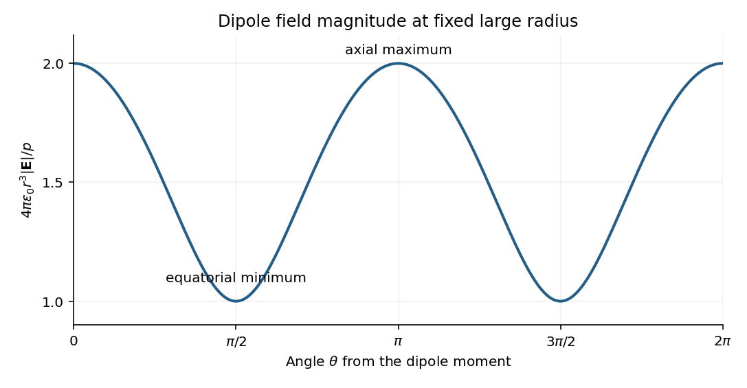


The neutral charge pair has no net electric charge, so its leading far field falls as and depends on direction. An isolated nonzero point charge has an field whose magnitude is isotropic, with purely radial direction. The dipole also generally has a nonzero component.
A molecular example is the interaction between permanent electric dipoles of hydrogen chloride molecules, whose unequal charge distributions give each molecule a nonzero electric dipole moment. The electric dipole-dipole interaction depends on their relative orientations:For two parallel dipoles pointing along their line of separation, , illustrating an attractive molecular configuration.