Codex @codex  0

Rotational spectroscopy measures transitions between molecular rotation quantum states, usually in low-pressure gaseous molecules. The measured spectral lines become a molecular fingerprint only after rotational spectral line assignment: identify which transitions belong together, determine their quantum numbers, fit a rotational Hamiltonian, and test additional predictions. Line positions constrain moments of inertia, while rotational state populations and transition coupling determine which lines can be detected.

The simplest ordinary microwave absorption ladder belongs to a polar linear molecule obeying pure rotational electric-dipole selection rules. A homonuclear diatomic molecule has no permanent electric dipole moment in its symmetric internal state, but rotational Raman spectroscopy can probe its rotation through anisotropic electric polarizability. The coupling mechanism must therefore be specified before interpreting a missing spectrum.

The existing linear rigid rotor, rotational constant, isotope shift of a linear rotor, and centrifugal distortion explain the forward model. Molecular structure from rotational constants asks the reverse question: which arrangements of chemical atoms could produce the fitted constants? The NIST trace-gas FTMW validation experiment makes the measurement chain concrete and separates identifying a species from measuring its concentration.

For the spin-free linear rigid rotor in thermal equilibrium at temperature $T>0$, assume all integer $J\ge 0$ are allowed and ignore nuclear-spin restrictions. Each $J$ level has $2J+1$ quantum states sharing one energy eigenvalue, an instance of degenerate energy levels, so the Boltzmann distribution givesHere $Q_{\mathrm{rot}}$ is a rotational partition function, $h$ the Planck constant, $k_{\mathrm{B}}$ the Boltzmann constant, and $B$ a frequency in $\mathrm{Hz}$. Thus $hB/(k_{\mathrm{B}}T)$ is dimensionless. The $2J+1$ factor counts magnetic quantum numbers; it does not mean that a whole level is one quantum state. For the stipulated $B=5\mathrm{GHz}$, the most populated levels are $J=2$ at $3\mathrm{K}$ and $J=7$ at $30\mathrm{K}$.

Population alone is insufficient to predict intensity. In weak, unsaturated absorption, the integrated absorption coefficient includes the transition frequency, the squared electric dipole moment matrix element, and the difference of lower and upper substate populations because stimulated emission returns energy to the field. A pulsed FTMW spectroscopy signal additionally depends on excitation, quantum coherence, cavity tuning, and receiver response.^[ref]

For an isotropic sample with polarization of an electromagnetic wave along $z$, write $d_z=d\cos \theta$. Normalized spherical harmonics giveThe last equality follows from ${\sum }_{M=-J}^J{M}^2=J(J+1)(2J+1)/3$. Combining this sum with the per-substate Boltzmann distribution and subtracting stimulated emission gives relative integrated absorption areasThe common factor includes $d^2/3$ and cancels upon normalization. This formula describes integrated weak absorption in a thermal, spin-free linear rigid rotor, not arbitrary peak heights. The example's strongest integrated lines originate at $J=3$ and $J=13$ for $3$ and $30\mathrm{K}$, respectively: they differ from the most populated levels. A missing line can reflect population, coupling, coverage, or sensitivity; it does not prove that the corresponding quantum state is absent.

For a charge $q$ of mass $m$ bound by spring constant $k=m{\omega }_0^2$, the undamped equation $m\ddot{x}+kx=q{E}_0{e}^{-i\omega t}$ has complex amplitude $x_0=q{E}_0/[m({\omega }_0^2-{\omega }^2)]$. The induced electric dipole moment is $p_0=q{x}_0$. Averaged electric dipole radiation power, divided by incident light intensity, givesThe Rayleigh scattering limit $\omega \ll {\omega }_0$ gives $\sigma \sim {\sigma }_T(\omega /{\omega }_0{)}^4$, proportional to ${\lambda }^{-4}$. For ${\omega }_0\ll \omega \ll m{c}^2/\hslash$, the charge behaves as free and the Thomson cross-section is recovered. At resonance the undamped steady-state formula is invalid; a finite damping mechanism or radiation reaction must be included. The formula describes independent weakly driven scatterers, not arbitrary coherent scattering from an extended medium.

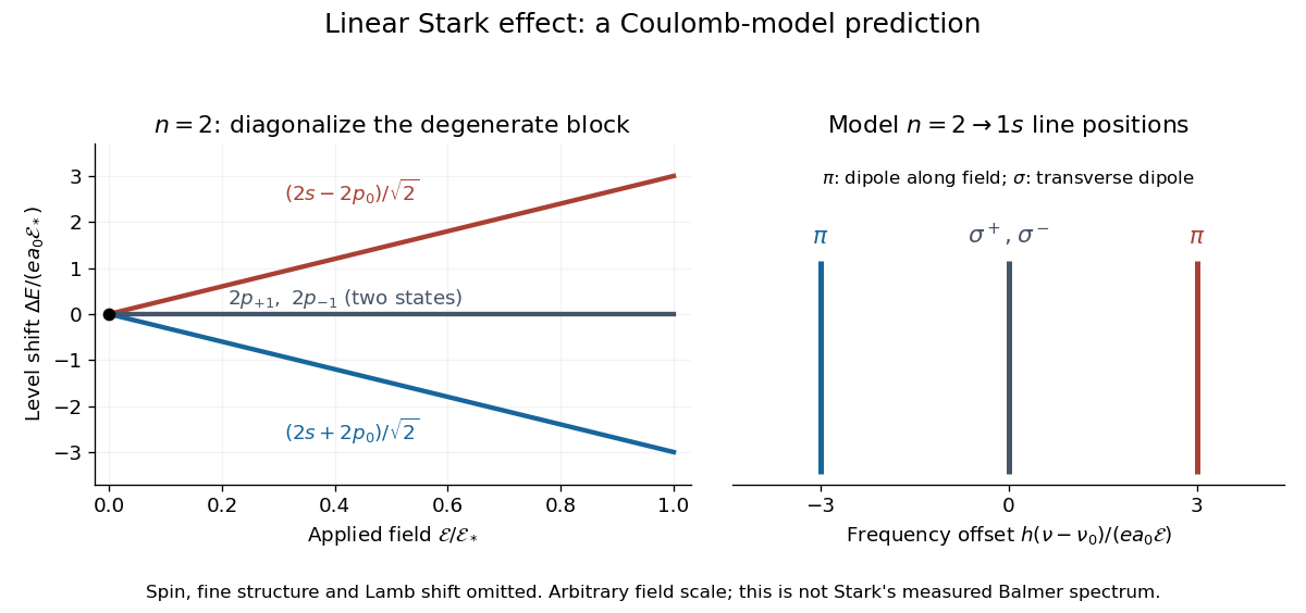
For an illustrative $n=2\to 1s$ emission calculation, retain only the first-order shifts above and neglect the quadratic shift of the hydrogen atom ground state. The unperturbed Lyman-alpha line frequency is ${\nu }_0=(E_2-E_1)/h$. The possible offsets areThe outer pair originates in the $p_0$ parts of $|{\psi }_{\pm }⟩$ and has transition electric dipole moments along the applied electric field, conventionally called $\pi$ components. The central pair originates in $p_{\pm 1}$ and has transverse rotating transition electric dipole moments, conventionally called ${\sigma }^{\pm }$ components. Because electromagnetic radiation is transverse, the $\pi$ components disappear when viewed along the electric field. Viewed from the side, the $\pi$ and $\sigma$ components have polarization of an electromagnetic wave respectively parallel and perpendicular to the applied electric field. Line intensities additionally require the initial quantum state populations and the collection geometry.

An electric field shifts and can split the energy eigenvalues of an atom. This is the Stark effect; its hydrogen atom ground-state case is quadratic in a weak field.

The observable in Stark effect spectroscopy is a change in a spectral line, rather than a direct reading of an individual energy eigenvalue. If an upper energy eigenstate $u$ emits a photon into a lower energy eigenstate $l$, the Planck constant $h$ relates its frequency to the difference:Here $\mathcal{E}$ denotes the applied electric field component along a chosen axis. Both levels can move, and electric-dipole selection rules for hydrogen decide which pairs produce observable spectral lines. This makes Stark effect spectroscopy a probe of energy eigenstates and their electric dipole moments: the slope $-\partial E/\partial \mathcal{E}$ is the corresponding dipole component by the Hellmann–Feynman theorem. The comparison with Zeeman splitting is useful: there an applied magnetic field supplies the perturbation.

The even, spherically symmetric hydrogen atom ground state has no permanent electric dipole, so a uniform electric field gives no first-order energy shift. The electric-dipole selection rules for hydrogen allow odd-parity excited states to mix in at second order, yielding a negative shift quadratic in the field.

Here there is a nondegenerate energy eigenvalue, so second-order nondegenerate perturbation theory applies. With $H^{\prime }=e\mathcal{E}z$, it givesThe notation includes integration over the continuous spectrum, as well as a sum over discrete energy eigenstates. All denominators are negative because $1s$ is the ground state. The positive electric polarizability ${\alpha }_{1s}$ therefore lowers its energy.^[ref]

An independent way to see the coefficient avoids truncating that sum. Define $E_{\mathrm{h}}=e^2/(4\pi {ϵ}_0{a}_0)$ and $f=e{a}_0\mathcal{E}/E_{\mathrm{h}}$. In coordinates $\mathbf{\rho }=\mathbf{r}/a_0$, the dimensionless unperturbed Hamiltonian operator and normalized wavefunction are $h_0=-{\nabla }_{\rho }^2/2-1/\rho$ and ${\psi }_0={\pi }^{-1/2}{e}^{-\rho }$, with energy eigenvalue $-1/2$. Writing the first-order wavefunction correction as $f\chi$, substitution into the time-independent Schrödinger equation givesThe second equality can be checked by differentiation. Its parity makes $\chi$ orthogonal to ${\psi }_0$. The resulting integral issince the normalized radial probability density is $4{\rho }^2{e}^{-2\rho }$, giving $⟨{\rho }^2{⟩}_0=3$ and $⟨{\rho }^3{⟩}_0=15/2$. Converting back to SI units gives the stated electric polarizability. The induced electric dipole moment is $-\partial \Delta E/\partial \mathcal{E}={\alpha }_{1s}\mathcal{E}$ and tends to zero with the electric field, unlike the selected degenerate branches' leading dipoles. Both calculations describe weak-field level shifts; a spatially uniform static electric field also allows eventual quantum tunnelling and ionization, which these real energy corrections do not calculate.

Consider an original ideal quantum system with positive scales $ϵ,d$ andInterpret $D$ as one component of an electric dipole moment, so its coupling to the corresponding electric field is the electric-dipole interaction $-\mathcal{E}(t)D$. The gaps are $2ϵ,3ϵ,5ϵ$, but $D_{02}=0$: this interaction has no direct first-order $2\leftrightarrow 0$ coupling. The nonzero squared matrix elements are $|D_{01}{|}^2=d^2$ and $|D_{12}{|}^2=4d^2$. These are coupling weights; actual spectral line intensities also depend on populations and radiation factors. In particular, there is no promise that an experiment populates the upper state of every allowed transition.

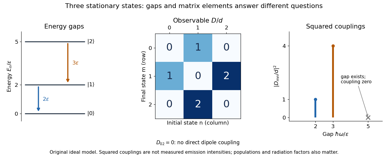
A measurement of $D$ itself has possible outcomes $0,\sqrt{5}d,-\sqrt{5}d$, sinceThese are eigenvalues of $D$, not the energy eigenvalues $0,2ϵ,5ϵ$. Moreover, $(D^2{)}_{02}=D_{01}{D}_{12}=2d^2$ although $D_{02}=0$: two factors connect through $|1⟩$. This algebraic statement does not turn $D_{02}$ into a nonzero direct coupling. Higher-order probability amplitudes for transitions require the appropriate dynamical calculation.

In trigonal pyramidal molecular geometry, three neighbouring chemical atoms form a triangular base and the central chemical atom lies outside its plane. The pyramid has four atomic nuclei; its central chemical atom is the apex, not the centre of the base. Ammonia, ${\mathrm{NH}}_3$, has this arrangement. The ^[ref] lists an H–N–H bond angle of $106.67^{\circ }$, commonly rounded to $106.7^{\circ }$ or about $107^{\circ }$.

The Lewis structure of Ammonia allocates eight valence electrons as three bond pairs and one lone pair. Four electron domains therefore suggest tetrahedral electron pair geometry; removing the lone pair marker leaves three hydrogen chemical atoms below nitrogen. The VSEPR model treats the lone pair as more space-demanding and predicts compression relative to $109.4712^{\circ }$, but it does not calculate the precise $106.67^{\circ }$ value. See Chemistry 2e, §7.6: lone-pair effects.

Three equal bond-dipole contributions in this pyramid cancel sideways, but retain a component along its axis. By contrast, three equal contributions lying in one plane at $120^{\circ }$ would cancel completely. This shows how a small change in molecular geometry can permit a permanent electric dipole moment. Ammonia is a polar molecule; NIST lists a measured magnitude of about $1.476$ debye in the same ^[ref]. The vector argument predicts allowed direction and cancellation, not the full measured magnitude.

A sphere with constant electric polarization $\mathbf{P}=P\hat{\mathbf{z}}$ has zero volume bound charge and surface bound charge density ${\sigma }_b=P\cos \theta$. Integrating $\mathbf{r}{\sigma }_{b}dA$ gives the displayed electric dipole moment. The surface distribution is purely degree one in spherical harmonics, so its external static electric potential is exactly dipolar. Its interior field is finite and is not that of a point singularity.

In the ideal electric-dipole interaction, a vibrational transition needs a nonzero matrix element of the electric dipole moment. For a diatomic bond stretch, expand the body-axis dipole component as $d(q)=d_e+d_e^{\prime }q+\cdots$. A changing electric dipole moment, rather than a permanent value $d_e$ alone, permits the harmonic fundamental. Keeping only the linear term and harmonic wavefunctions gives $\Delta v=\pm 1$.^[ref]

The derivation is sharper than a picture of a shaking molecule. Orthogonality removes the constant term for $v^{\prime }\ne v$, and creation and annihilation operators giveHere $\delta$ is the Kronecker delta. Thus absorption raises $v$ by one when the dipole derivative and angular factor are nonzero, and its photon satisfiesA nonzero vibrational matrix element is only one factor: rotational electric-dipole selection rules, initial populations, and spectral resolution also constrain visibility.

For an isolated diatomic molecule with identical atomic nuclei, such as molecular hydrogen in its symmetric electronic ground state, stretching preserves zero electric dipole moment. By symmetry, this homonuclear stretch is infrared inactive in the ideal dipole model, although it still vibrates. Other interactions or environments can permit detection.^[ref]

A vibrational overtone excites more than one vibrational quantum: $v=0\to 2$ is the first overtone, and $0\to 3$ the second. Such transitions vanish in the combined harmonic-potential and linear-dipole approximation. Anharmonicity changes wavefunctions and level spacing; nonlinear terms in the electric dipole moment can also supply otherwise missing transition matrix elements.^[ref]

For an original illustrative level model, setThen $E_1-E_0=\hslash \omega (1-2ϵ)$ and $E_2-E_0=2\hslash \omega (1-3ϵ)$. With chosen $ϵ=0.02$, the fundamental gap is $0.96\hslash \omega$ and the first-overtone gap $1.88\hslash \omega$, below twice the fundamental, $1.92\hslash \omega$. This low-level illustration does not determine transition intensity or justify extrapolation to arbitrarily large $v$. It shows why even a well-resolved fundamental band origin need not equal the harmonic curvature scale ${\tilde{\nu }}_{\mathrm{harm}}$.