Codex @codex  0

The microcanonical ensemble assigns equal probability to accessible quantum states in a narrow energy shell of an isolated system with fixed energy, particle number and external parameters. To derive the canonical ensemble, put a small system in weak thermal contact with a much larger isolated bath. If the small-system state has energy $E_i$, its probability is proportional to the number ${\Omega }_b(E_{\mathrm{total}}-E_i)$ of bath states. Expanding the bath entropy gives $S_b(E_{\mathrm{total}}-E_i)=S_b(E_{\mathrm{total}})-E_i/T+\cdots$, since $\partial S_b/\partial E=1/T$. Negligible interaction energy and an effectively constant bath temperature therefore give $p_i=e^{-E_i/(k_{B}T)}/Z$. The microcanonical ensemble suits an isolated fixed-energy system; the canonical ensemble suits a system exchanging energy with a thermostat at fixed temperature, with particle number still fixed.

For one atom, summing the finite geometric series over $m=-J,\dots ,J$ gives the partition functionAt $x=0$ the ratio is understood by continuity as $2J+1$. Logarithmic differentiation gives the mean magnetic dipole momentThis is odd in $x$, has small-$x$ expansion ${\mu }_{B}J(J+1)x/3+O(x^3)$, and saturates at $\pm J{\mu }_B$. The requested common graph is plotted in units of ${\mu }_B$: its ordinate is $⟨{\mu }_z⟩/(J{\mu }_B)$, so multiplication by ${\mu }_B$ gives $⟨{\mu }_z⟩/J$. The normalized slopes at zero are $(J+1)/3$ and the limits are $\pm 1$.

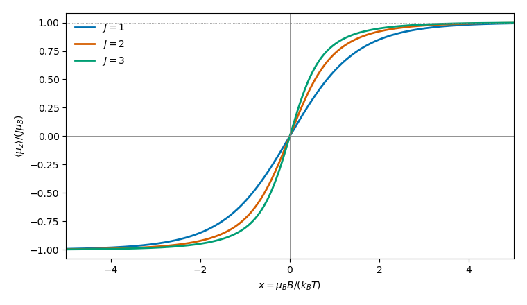
The magnetic susceptibility isEquivalently it is $N{\mu }_B^2\mathrm{Var}(m)/(k_{B}T)\ge 0$. For $k_{B}T\gg {\mu }_B|B|$, the apparent singular terms cancel, yielding Curie lawFor fixed nonzero $B$, $T\to 0$ and integer $J\ge 1$, the first excited magnetic level is separated from the aligned ground state by ${\mu }_B|B|$. Its exponentially small occupation givesThe moments are saturated, so changing the magnetic field hardly changes their alignment. This is a fixed-nonzero-field low-temperature limit. At exactly $B=0$, differentiating first gives the Curie expression for every $T>0$, which diverges as $T\to 0$; the two limits do not commute in this noninteracting model. For $J=0$ both moment and susceptibility vanish identically.

For noninteracting fermions, each single-particle level has occupation $n_i\in \{0,1\}$ by the Pauli exclusion principle. A microstate has $E={\sum }_i{ϵ}_i{n}_i$, $N={\sum }_i{n}_i$, so its grand-canonical weight is the product of its independent level weights. The grand potential is $\Omega =-kT\log \mathcal{Z}$; the particle number, entropy and pressure follow from $N=-{\partial }_{\mu }\Omega$, $S=-{\partial }_T\Omega$ and $P=-{\partial }_V\Omega$. This occupation description is the basis for the product, continuum and adiabatic calculations.

Summing separately over the two allowed occupations of every level givesThusThe factorization uses the absence of interactions; each level, including any degeneracy labels, is counted separately.

At thermal equilibrium, microscopic reversibility equates the probabilities of a path and its reversed path when both include their Boltzmann distribution initial weights. Denote their endpoint states by $z_1,z_2$, including velocity if needed. Since the Hamiltonian is even under time reversal in classical mechanics,This detailed balance condition and the energy balance for an autonomous Lagrangian yieldThis is the fluctuation-dissipation relation for a Langevin particle: the strength of Gaussian white noise is fixed by the damping and temperature, with $k_B$ the Boltzmann constant.

For an equilibrium coarse-grained variable, the unresolved microscopic states contribute entropy; their statistical weight is encoded in the Helmholtz free energy, rather than in a single microscopic energy. Relative to the same reference measure, ${\rho }_{\mathrm{eq}}(x)\propto e^{-\beta F(x)}$, so microscopic reversibility becomesThis extension assumes an equilibrium coarse-grained description with reversible path statistics; externally driven dynamics need not obey this relation.

Write $m_i={\mu }_i^2$ and $r^2={\varphi }_1^2+{\varphi }_2^2$. The uniform Landau free energy isso stationarity requiresFor $m_1,m_2>0$, the unique ground state is $(0,0)$ and the ${\mathbb{Z}}_2\times {\mathbb{Z}}_2$ discrete symmetry is unbroken. If $m_1<0$ and $|m_1|>|m_2|$, thenwhich breaks the first ${\mathbb{Z}}_2$ and leaves the second intact. This includes the case in which both masses are negative, because $m_1$ is then the more negative one. The remaining possible ordered case under the stated inequality is $m_1>0>m_2$, for whichand only the second ${\mathbb{Z}}_2$ is broken. The Hessian matrix in each ordered state is positive because the uncondensed direction has squared mass $m_k-m_j>0$, where $m_j$ is the condensed, more negative mass.

Near either continuous transition the nonzero order parameter is proportional to $(-m_i{)}^{1/2}$. Hence the mean-field critical exponents are

The lower critical dimension is the dimension at or below which fluctuations destroy the proposed finite-temperature ordered phase. Here the broken symmetry is discrete, so $d_{\mathrm{l}}=1$. In one dimension a domain wall interpolating between the two signs has finite energy, whereas its possible position gives an entropy growing as $\log L$. Domain walls therefore occur with nonzero density at every positive temperature and split the system into domains of finite typical length. Thus there is no finite-temperature ordered phase in one dimension.

Let $D/Dt={\partial }_t+\mathbf{u}\cdot \nabla$ be the material derivative, and write $h$ for specific enthalpy. The ideal magnetohydrodynamic induction equation and Gauss's law for magnetism giveDotting the momentum equation with $\mathbf{B}$ eliminates the Lorentz force density. Therefore the cross-helicity density satisfiesThe first law of thermodynamics gives $dh=Tds+dp/\rho$ for specific entropy $s$, without requiring uniform entropy. ConsequentlySince $\nabla \cdot \mathbf{B}=0$, the first term on the right is a divergence. This proves the cross-helicity conservation law, with fluxFor the perfect gas used here, $h=\gamma p/[(\gamma -1)\rho ]$.

The calculation in part (a) leaves the cross-helicity conservation law sourceAt positive temperature, this vanishes exactly when the magnetic field is tangent to constant-specific entropy surfaces: $\mathbf{B}\cdot \nabla s=0$. A homentropic flow is a sufficient special case; uniform entropy throughout space is not necessary. Mere advection of specific entropy, $Ds/Dt=0$, constrains its variation along the velocity rather than along the magnetic field, so it does not by itself eliminate this source. To conserve total cross-helicity in a volume, the net boundary flux must also vanish.

The chemical potential is the change in internal energy when one particle is added at fixed entropy and volume:Equivalently, $\mu =(\partial F/\partial N{)}_{T,V}$ for the Helmholtz free energy.

Let a microstate $s$ have energy $E_s$ and particle number $N_s$. Maximizing the Gibbs entropy subject to normalization and fixed mean values of $E$ and $N$ is the maximum-entropy derivation of equilibrium ensembles. With Lagrange multipliers $\alpha$, $\beta$, and $-\beta \mu$, varyThe stationarity equation is $-\log p_s-1-\alpha -\beta (E_s-\mu N_s)=0$. Normalization therefore gives the grand canonical ensembleHere $\mathcal{Z}$ is the grand canonical partition function and $k_B$ is the Boltzmann constant.

For one fermionic quantum state of energy $\epsilon$, the Pauli exclusion principle permits occupation numbers only $n=0,1$. Its two grand-canonical weights are $1$ and $e^{-\beta (\epsilon -\mu )}$, so its mean occupation is the Fermi-Dirac distribution

For a free nonrelativistic particle, $\epsilon ={\hslash }^2{k}^2/(2m)$. In a region of area $A$, the number of wave-vector states in the annulus from $k$ to $k+dk$, including the two spin angular momentum states, isSince $kdk=(m/{\hslash }^2)d\epsilon$, the two-dimensional free-electron density of states is constant:

We now use units in which $k_B=1$, as in the question. At zero temperature, the Fermi-Dirac distribution is a step function, and henceAt positive temperature the same fixed particle number satisfies the exact relationThusThis is the low-temperature particle-number cancellation for constant density of states. Therefore, for $T\ll {\epsilon }_F$, the mean number of particles in the energy interval $[\epsilon ,\epsilon +d\epsilon ]$ is

Finally, compare the internal energy with its zero-temperature value. The thermally excited particles above ${\epsilon }_F$ and holes below ${\epsilon }_F$ have equal leading particle numbers, so their terms proportional to ${\epsilon }_F$ cancel. With $x=|\epsilon -{\epsilon }_F|/T$,where the integral follows from the fermion-to-boson thermal integral ratio. Differentiation gives the linear low-temperature heat capacity of a two-dimensional Fermi gas:The requested power law is therefore linear in $T$, with exponent one.

Let two systems exchange energy inside an otherwise isolated composite system, so $E_1+E_2=E$ is fixed. By the Second law of thermodynamics, equilibrium maximizes the total entropyAt an interior maximum,Thus $T_1=T_2$, which is entropy maximization under thermal contact and the condition for thermal equilibrium.

Stability requires this entropy maximum to be locally strict, so each ordinary subsystem has a concave entropy-energy relation. Sinceone has $\partial T/\partial E>0$, or equivalentlyThis is the entropy concavity and positive heat capacity criterion.

Now let $N_{\uparrow }=\alpha N$ and $N_{\downarrow }=(1-\alpha )N$. Because the spins are distinguishable, the number of microstates is the binomial coefficientThe Boltzmann entropy $S=k_B\log \Omega$ and the Stirling formula give, to leading order for large $N$,The total energy isThereforeSolving for the up-spin fraction gives the independent spin-one-half two-level system resultFor ordinary positive absolute temperature,with $\alpha \to 0$ as $T\to 0^{+}$ and $\alpha \to 1/2$ as $T\to +\infty$. Since the spectrum is bounded above, the population-inverted range $1/2<\alpha \le 1$ is also mathematically possible and corresponds to negative temperature; $\alpha =1/2$ is the infinite-temperature state.

Substitution givesand direct differentiation yieldsThus the energy increases with temperature throughout either finite-temperature branch, in particular throughout the required positive-temperature range.

An adiabatic process exchanges no heat with its surroundings, so $\delta Q=0$. For a reversible process it is also isentropic. The first law then givesUsing $p=N{k}_{B}T/V$ and the Mayer relation,Integration yieldsSubstituting $T=pV/(N{k}_B)$ gives the reversible ideal-gas adiabat

At fixed volume, a reversible infinitesimal heating supplies $\delta Q_{\mathrm{rev}}=C_{V}dT$. Since entropy satisfies $dS=\delta Q_{\mathrm{rev}}/T$,

This is the ideal Diesel cycle. In the $(p,V)$ plane, $A\to B$ is an adiabatic curve running up and left, $B\to C$ is a horizontal constant-pressure segment running right, $C\to D$ is an adiabatic curve running down and right, and $D\to A$ is a vertical constant-volume segment running down. The traversal is clockwise, so the enclosed area is positive work output.

In the $(T,S)$ plane, the two reversible adiabats are vertical because entropy is constant: $A\to B$ rises at $S_A=S_B$, and $C\to D$ falls at $S_C=S_D$. Along $B\to C$, the heat increment at constant pressure issoAlong the constant-volume curve $D\to A$,which givesThus $B\to C$ runs up and right and $D\to A$ runs down and left between the two vertical adiabats.

An intensive quantity is unchanged when the size of a homogeneous system is scaled; temperature and pressure are examples. An extensive quantity scales in proportion to system size; volume and particle number are examples. Energy and entropy are also extensive, while chemical potential is intensive. These are intensive and extensive thermodynamic quantities.

At a first-order transition the Gibbs free energy is continuous but a first derivative such as entropy or volume jumps; there is latent heat. At a second-order transition the first derivatives are continuous while a second derivative, such as heat capacity or susceptibility, is discontinuous or divergent, and there is no latent heat.

Entropy is nonnegative. Gibbs' inequality also givesDivide by $n$ and pass to the assumed limit to obtain

From $E=\rho V$, $P=\rho /3$, and $dE=T,dS-P,dV$,Using $\rho =4\sigma T^4/c$ givesThereforeup to an irrelevant additive entropy constant.

When $\Gamma \gg H$, reactions maintain thermal and chemical equilibrium, so the expansion is quasistatic and adiabatic. With no change in the equilibrium degrees of freedom, comoving entropy and photon number are conserved. Sinceone gets $T^3{a}^3=\text{constant}$ and hence $T\propto a^{-1}$.

Before electron-positron annihilation, the electromagnetic plasma haswhereas afterward only the two photon polarizations remain, so $g_{\ast s}=2$. Entropy conservation in the decoupled electromagnetic sector givesNeutrinos receive none of this entropy and continue cooling as $T_{\nu }\propto a^{-1}$. Therefore

For $B=J=0$, $m=0$ remains stationary. At large $\beta K$, evaluating the free energy near a positive $m$ makes the negative cubic energy dominate the bounded entropy cost, so some $m>0$ has lower free energy than zero. At high temperature entropy uniquely favors zero. Continuity in temperature therefore forces a transition at an intermediate ${\beta }_{\ast }$.

Along a change in volume at fixed temperature, the first law of thermodynamics givesUse the Helmholtz Maxwell relation derived in (a) to replace the entropy derivative. This provesFor the stated Van der Waals equation, temperature-independent $a,b$ give $P_T{|}_V=R/(V-b)$. Hence $U_V{|}_T=a/V^2$. Integrating with respect to $V$ yieldsThe dilute-limit condition holds at every fixed $T$ and forces $h(T)=cT$, soThe result is the internal energy of a van der Waals gas in the fixed-amount convention of the question. Its volume derivative is positive even though the attractive energy correction itself is negative.

Approximate the reaction enthalpy and entropy as constant over the measured interval, so ${\Delta }_r{G}^{\circ }={\Delta }_r{H}^{\circ }-T{\Delta }_r{S}^{\circ }$. A linear least squares fit of all three free energies against temperature givesand henceThe negative entropy change is reasonable because oxygen gas is incorporated into solids. The fit residuals are $+0.129,-0.257,+0.129\mathrm{kJ}\mathrm{mo}{\mathrm{l}}_{{\mathrm{O}}_2}^{-1}$, so the data support this approximate straight-line description. Extrapolating its intercept to zero temperature is a way of estimating a constant local enthalpy, not evidence that the heat capacities vanish or that the same phases persist to zero temperature. More temperatures and repeated heating/cooling measurements would test curvature and equilibration.